Change Gridline / Cell Border Color in Excel & Google Sheets

This tutorial demonstrates how to change the cell border color in Excel and Google Sheets.

 

Change Gridline Color

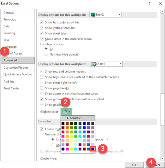
1. To change the gridline color, in the Ribbon, go to File > Options.

2. This brings up the Excel Options window. Go to Advanced > Display options for this worksheet.
   Then click the paint icon next to Gridline color, choose a color, and click OK.

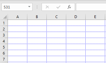
Now the gridline color is blue, as you can see below.

Tip: For more options related to gridline display, see What Are Gridlines?

Change Cell Border Color

Format Cells

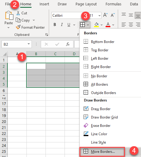
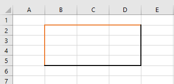
Say you have a list of the data range (here, B2:D5) with a border around it. To change the border color (here, from black to orange), follow these steps:

1. First, select the cells where you want to change the border colors. Then in the Ribbon, go to Home > Font. Click the Borders icon and choose More Borders…

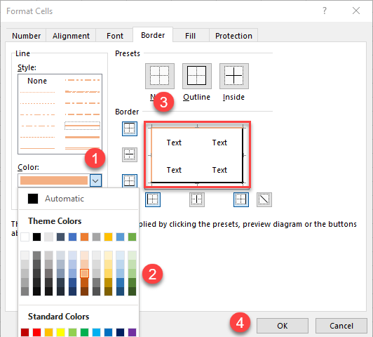
2. This brings up the Format Cells window. Under Color, choose from the drop down.
   To the right, in the preview diagram, click the individual Border sides (or Presets) to set which borders you want. Then click OK.

As a result, the border color is changed.

Border Command

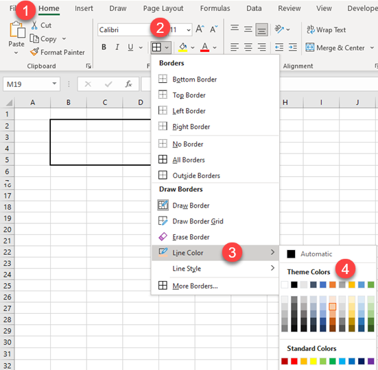
1. In the Ribbon go to Home > Font. Click the Borders icon and choose Line Color. Then choose a color for the border.

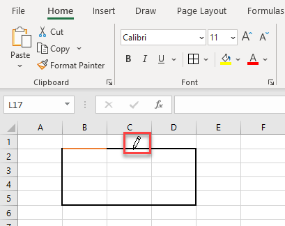
2. The cursor changes to a pencil. Use it to click each part of the border to change its color.

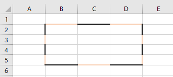
As a result, parts of the border are a different color.

Tip: You can also use VBA code to set cell border color.

Change Cell Border Color in Google Sheets

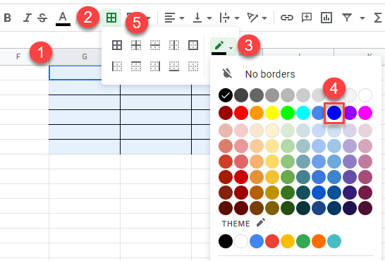
1. First select the cells where you want to change the border color.
2. Then in the Toolbar, click the Borders icon.
3. Click the Change Color icon.
4. Then choose a color.
5. To finish, set the border style for the cell.

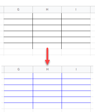
Now the borders are blue.

Unfortunately, you can’t change the default color of the gridlines in Google Sheets.