IFERROR Function in Excel, VBA, & Google Sheets **Updated 2022**
Written by
Reviewed by
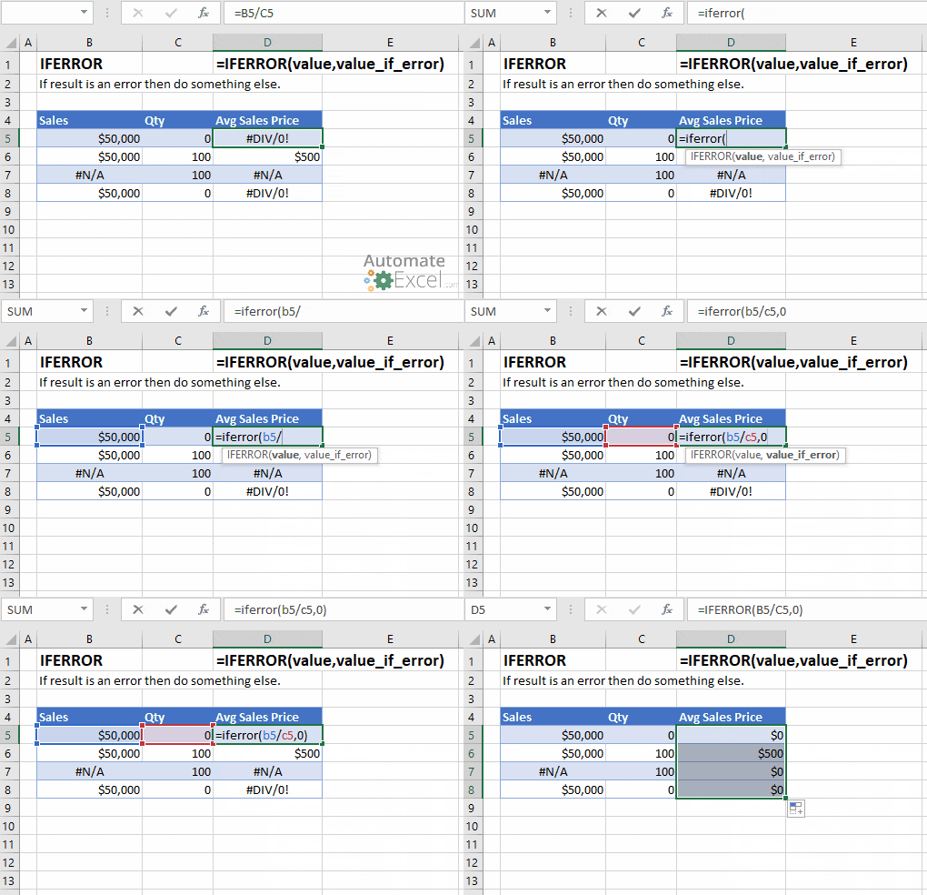
This tutorial demonstrates how to use the Excel IFERROR Function to catch formula errors, replacing them with another formula, blank value, 0, or a custom message.
What Is the IFERROR Function?
IFERROR allows you to perform a calculation. If the calculation does not result in an error, then the calculation result is displayed. If the calculation does result in an error then another calculation is performed (or a static value like 0, blank, or some text is outputted).
When would you use the IFERROR Function?
- When dividing numbers to avoid errors caused by dividing by 0
- When performing lookups to prevent errors if the value isn’t found.
- When you want to perform another calculation if the first results in an error (ex. Lookup a value in a 2nd table if it’s not found in the first table)
Un-handled formula errors can cause errors within your workbook, but visible errors also make your spreadsheet less visibly appealing.
If Error Then 0
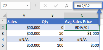
Let’s look at a basic example. Below you are dividing two numbers. If you attempt to divide by zero you will receive an error:
Instead, insert the calculation within the IFERROR Function and if you divide by zero a 0 is outputted instead of an error:
=IFERROR(A2/B2,0)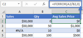
If Error Then Blank
Instead of setting errors to 0, you can set them to ‘blank’ with double quotations (“”):
=IFERROR(A2/B2,"")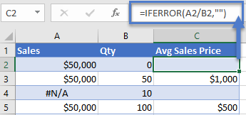
We will look at more IFERROR usages with the VLOOKUP Function…
IFERROR with VLOOKUP
Lookup functions like VLOOKUP will generate errors if the lookup value is not found. As shown above, you can use the IFERROR Function to replace errors with blanks (“”) or 0s:
=IFERROR(VLOOKUP(A2,LookupTable1!$A$2:$B$4,2,FALSE),"not found")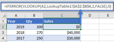
If Error Then Do Something Else
The IFERROR Function can also be used to perform a 2nd calculation if the 1st calculation results in an error:
=IFERROR(VLOOKUP(A2,LookupTable1!$A$2:$B$4,2,FALSE),
VLOOKUP(A2,LookupTable2!$A$2:$B$4,2,FALSE))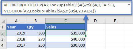
Here if the data is not found in ‘LookupTable1’ a VLOOKUP is performed on ‘LookupTable2’ instead.
More IFERROR Formula Examples
Nested IFERROR – VLOOKUP Multiple Sheets
You can nest an IFERROR inside another IFERROR to perform 3 separate calculations. Here we will use two IFERRORs to perform VLOOKUPs on 3 separate worksheets:
=IFERROR(VLOOKUP(A2,LookupTable1!$A$2:$B$4,2,FALSE),
IFERROR(VLOOKUP(A2,LookupTable2!$A$2:$B$4,2,FALSE),
VLOOKUP(A2,LookupTable3!$A$2:$B$4,2,FALSE)))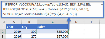
Index / Match & XLOOKUP
Of course, IFERROR will also work with Index / Match and XLOOKUP formulas as well.
IFERROR XLOOKUP
The XLOOKUP Function is an advanced version of the VLOOKUP function.
=IFERROR(XLOOKUP(A2,LookupTable1!$A$2:$A$4,LookupTable1!$B$2:$B$4),"Not Found")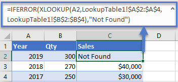
IFERROR INDEX / MATCH
INDEX and MATCH can be used to create more powerful VLOOKUPs (similar to how the new XLOOKUP function works) in Excel.
=IFERROR(INDEX(LookupTable1!$B$2:$B$4,MATCH(A3,LookupTable1!$A$2:$A$4,0)),"Not Found")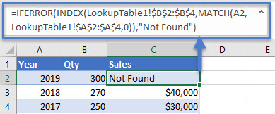
IFERROR in Arrays
Array formulas in Excel are used to perform several calculations through a single formula. Let’s suppose there are three columns of Year, Sales, and Avg Price. You can find out the total quantity with the following formula in the E column.
{=SUM($B$2:$B$4/$C$2:$C$4)}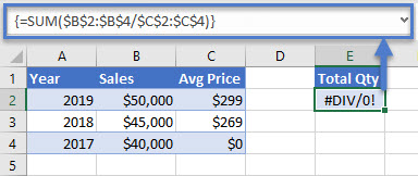
The formula performs well until it attempts to divde by zero, resulting in the #DIV/0! error.
You can use the IFERROR function like this to resolve the error:
{=SUM(IFERROR($B$2:$B$4/$C$2:$C$4,0))}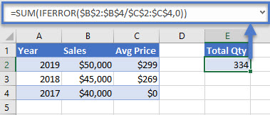
Notice that the IFERROR function must be nested inside the SUM Function, otherwise the IFERROR will apply to the sum total and not each individual item in the array.
IFNA vs. IFERROR
The IFNA Function works exactly the same as the IFERROR Function except the IFNA function will only catch #N/A errors. This is extremely useful when working with lookup functions: regular formula errors will still be detected, but no error will appear if the lookup value is not found.
=IFNA(VLOOKUP(A2,LookupTable1!$A$2:$B$4,2,FALSE),"Not Found")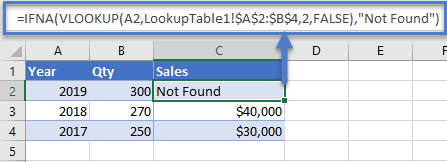
If ISERROR
If you are still using Microsoft Excel 2003 or an older version, then you can substitute IFERROR with a combination of IF and ISERROR. Here is a brief example:
=IF(ISERROR(A2/B2),0,A2/B2)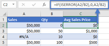
IFERROR in Google Sheets
The IFERROR Function works exactly the same in Google Sheets as in Excel:

IFERROR Examples in VBA
VBA does not have a built-in IFERROR Fucntion, but you can also access the Excel IFERROR Function from within VBA:
Dim n as long
n = Application.WorksheetFunction.IfError(Value, value_if_error)
Application.WorksheetFunction gives you access to many (not all) Excel functions in VBA.
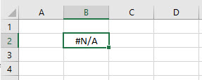
Typically IFERROR is used when reading values from cells. If a cell contains an error, VBA may throw an error message when attempting to process the cell value. Try this out with the example code below (where cell B2 contains an error):
Sub IFERROR_VBA()

Dim n As Long, m As Long

'IFERROR
n = Application.WorksheetFunction.IfError(Range("b2").Value, 0)

'No IFERROR
m = Range("b2").Value

End Sub
The code assigns cell B2 to a variable. The second variable assignment throws an error because the cell value is #N/A, but the first works fine because of the IFERROR function.
You can also use VBA to create a formula containing the IFERROR Function:
Range("C2").FormulaR1C1 = "=IFERROR(RC[-2]/RC[-1],0)"Error handling in VBA is much different than in Excel. Typically, to handle errors in VBA, you will use VBA Error Handling. VBA Error Handling looks like this:
Sub TestWS()
    MsgBox DoesWSExist("test")
End Sub

Function DoesWSExist(wsName As String) As Boolean
    Dim ws As Worksheet

    On Error Resume Next
    Set ws = Sheets(wsName)

    'If Error WS Does not exist
    If Err.Number <> 0 Then
        DoesWSExist = False
    Else
        DoesWSExist = True
    End If

    On Error GoTo -1
End Function
Notice we use If Err.Number <> 0 Then to identify if an error has occurred. This is a typical way to catch errors in VBA. However, the IFERROR Function has some uses when interacting with Excel cells.


