What Does the #REF Error Mean in Excel & Google Sheets?

This tutorial demonstrates how to find, interpret, and fix #REF! errors in Excel and Google Sheets.

 

 

Locate #REF! Cells in Excel

An #REF! error in Excel is a message that is displayed when a formula refers to an invalid cell. Usually, the cell is not valid because it was deleted or pasted over.

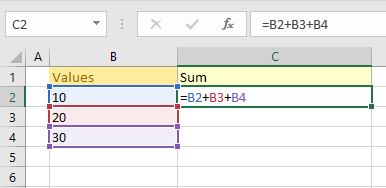
Say that, in cell C2, you have the formula:

=B2+B3+B4

 

 

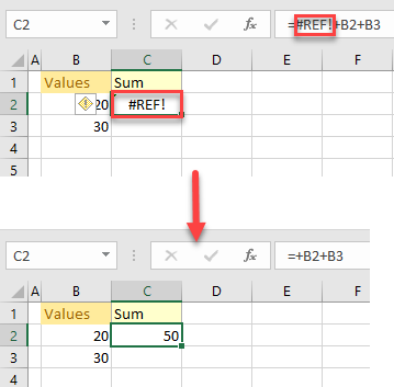
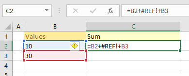
Suppose you deleted Row 3, causing the #REF! error.

 

 

Note: If you are referencing the cells as a continuous range (e.g., “=SUM(B2:B4)”), you won’t get a #REF! error after deleting a row or a column. Also, if you are specifically referencing cells and want to delete some of them, just delete the cell values. Don’t delete the whole row, and you won’t produce the #REF! error.

To locate the #REF! cells on your worksheet, just follow these steps:

1. In the Ribbon, go to Home > Find & Select > Go To Special.

 

 

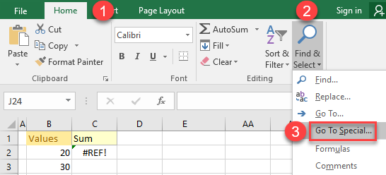
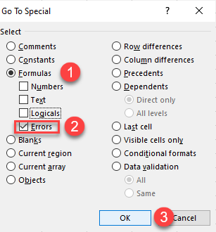
2. In the Go To Special window, choose Formulas and uncheck all boxes except Errors. Click OK.

 

 

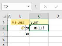
As a result, all the cells with the #REF! error message are selected.

 

 

Note: It’s also possible to cause a #REF! error by deleting a column or row, by having an incorrect row or a column reference in an INDEX Function, or by using incorrect range references in a VLOOKUP Function. Issues with OLE (Object Linking and Embedding), DDE (Dynamic Data Exchange), or macros can also cause the #REF! error.

Fix #REF! Errors

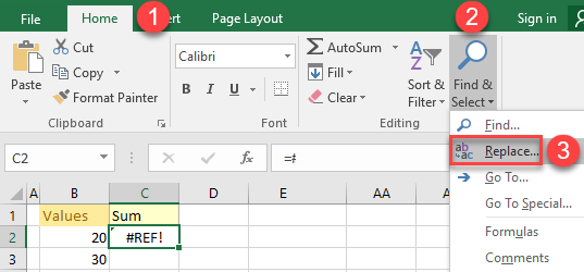
The best way to fix the problem above is to use the Find & Replace feature in Excel. Replacing the #REF! with blanks deletes the reference errors from your formulas.

1. In the Ribbon, go to Home > Find & Select > Replace (or use the CTRL + F shortcut to open the Find & Replace window).

 

 

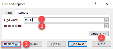
2. This opens the Find & Replace window. In the Find what: box type #REF! and Replace with: box leave empty. Then press Replace All and click Close.

 

 

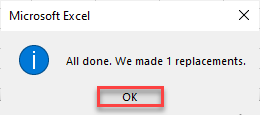
3. The pop-up information informs you how many replacements were made. To close it, click OK.

 

 

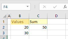
As a result, the #REF! error is fixed.

 

 

Other Potential Reasons For #REF! Error and Solutions

VLOOKUP With Incorrect Range Reference

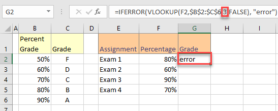
In this example, “=VLOOKUP(F2,$B$2:$C$6,3,FALSE)” returns the #REF! error, because it’s looking to return the value from the 3rd column, but the referenced range is $B$2:$C$6, which has only 2 columns. The solution is to correct the column lookup value to match the reference range (in this example: “=VLOOKUP(F2,$B$2:$C$6,2,FALSE)”).

 

 

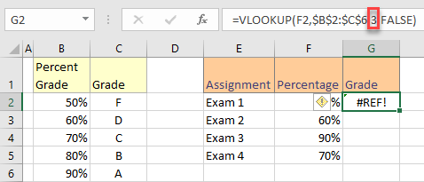
Another way to get rid of the #REF! error is to use the IFERROR Function. If there is an error in the formula the text from the function is displayed instead of #REF! (error in this example).

 

 

INDEX With Incorrect Row or Column Reference

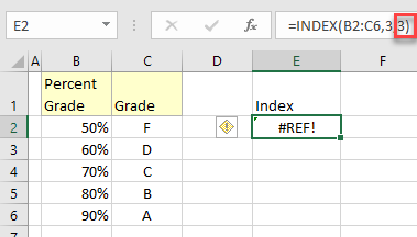
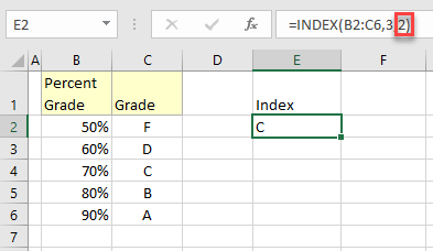
The #REF! error is displayed in this example (=INDEX(B2:C6,3,3)), because it’s looking to return the value from the 3^rd row, 3^rd column but the INDEX range is 5 rows by 2 columns. To correct this, choose a valid reference column (“=INDEX(B2:C6,3,2)”).

 

As a result, the #REF! error disappears, and cell E2 shows the correct value.

 

 

You can also use the IFERROR Function to get rid of #REF! error message.

Fix #REF! Errors in Google Sheet

#REF! errors in Google Sheets work very similar to those in Excel. In the case of a deleted cell causing the error, you can fix it with Find and replace.

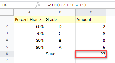
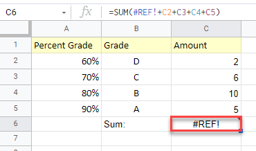
Say that, in cell C6, you have the formula:

=SUM(C2+C3+C4+C5+C6)

 

 

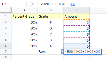
If you delete Row 3, for example, that causes a #REF! error.

 

 

To fix #REF! error in Google Sheets, follow these steps:

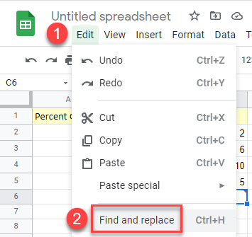
1. In the Menu, go to Edit and choose Find & Replace.

 

 

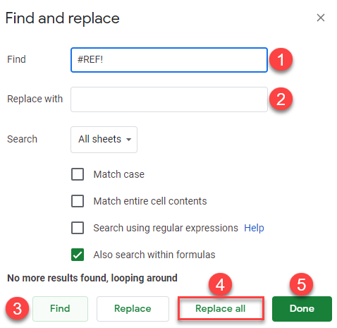
2. This opens the Find and replace window. In the Find box enter #REF! and the Replace box leave blank. After that, click Find and Replace All. Press Done.

 

 

As a result, the error is fixed.