Create Unique IDs in Excel & Google Sheets

This tutorial will demonstrate how to create unique IDs in Excel & Google Sheets.

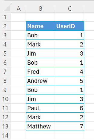
If you wish to create a unique identfier in Excel, you can use a combination of Excel functions to do so.   The entire formula that we will use is shown below:

=IF(ISNA(MATCH(B3,B2:$B$2,0)),MAX(C2:$C$2)+1,VLOOKUP(B3,B2:$C$2,2,FALSE))

MATCH Function

Taking a list of names, we can use the MATCH function to see what row the name is duplicated in the list

In the cell to the right of the first name of the list, we can type the following formula:

=MATCH(B3,$B$2:B2,0)

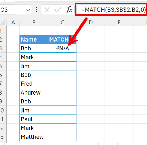
Then we can copy this formula down to the remaining list.

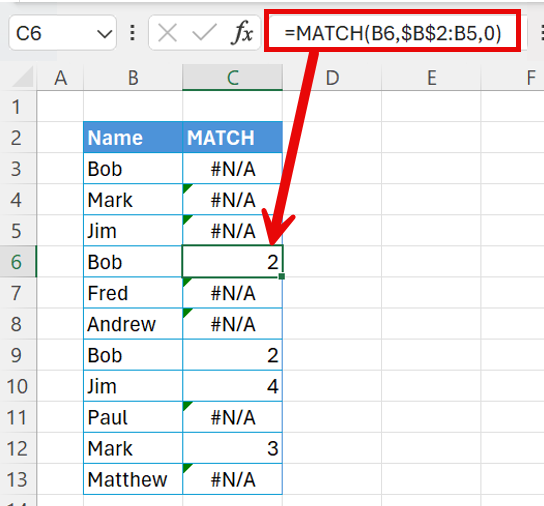
Note as soon as it finds a name that has already appeared in the list, it returns the row in the range that is being searched, otherwise it will return #N/A.  The formula above has an absolute reference within it. This means that when you copy the cell down, the cell reference that is locked will not change, while the other cell references will change to the relevant row they are copied to.  If you have a look at the graphics above, you will see that the cell B2 in the first formula has changed to cell B5. The range in the second formula is therefore including all the cells from B2:B5. As the formula is copied down, that range increases accordingly.

MAX Function

The next function that is used is the MAX function.  This function generates the unique number for us based on previous  unique numbers already generated.

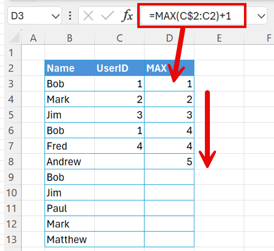
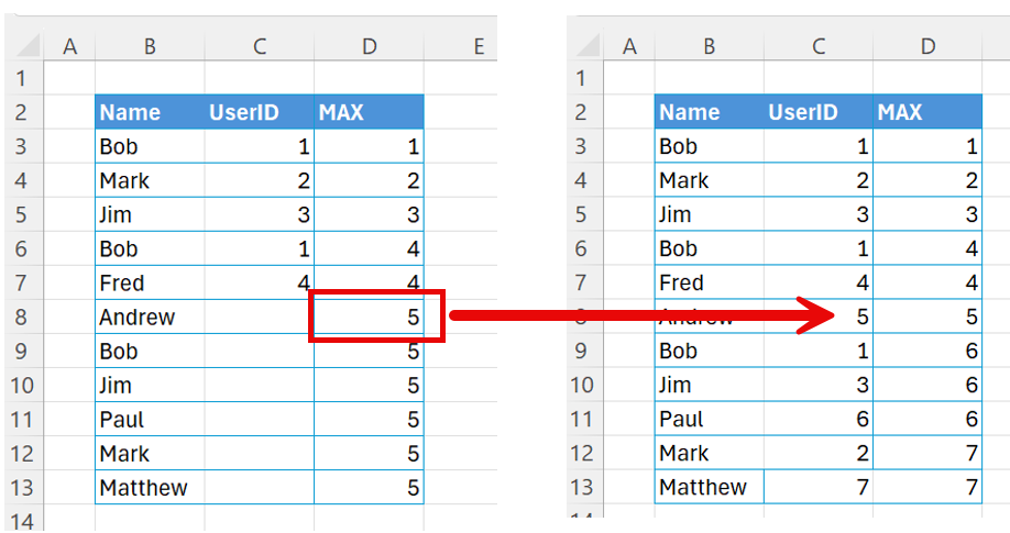
Our long formula has already generated the UserID’s 1 through to 4.   The MAX function contained in this formula would have produced these values.   As you can see in the graphics below, if the UserID has not been generated in Column C, then using the MAX value as a standalone function would give us the same value for the remaining rows – as 4 is the maximum value found and the formula is returning the MAX value PLUS 1.

ISNA Functions

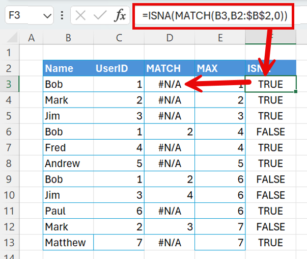
The ISNA function looks to see if a formula is returning a #N/A error.  If the formula is returning #N/A, then the ISNA function will return TRUE, otherwise it will return FALSE.

In our formula, we are using the ISNA function to see if the MATCH function returns #N/A.

=ISNA(MATCH(B3,B2:$B$2,0))

VLOOKUP Function

The VLOOKUP function is used to see if the value in column B has already been found, and if it has been found, it will return the value in column C.

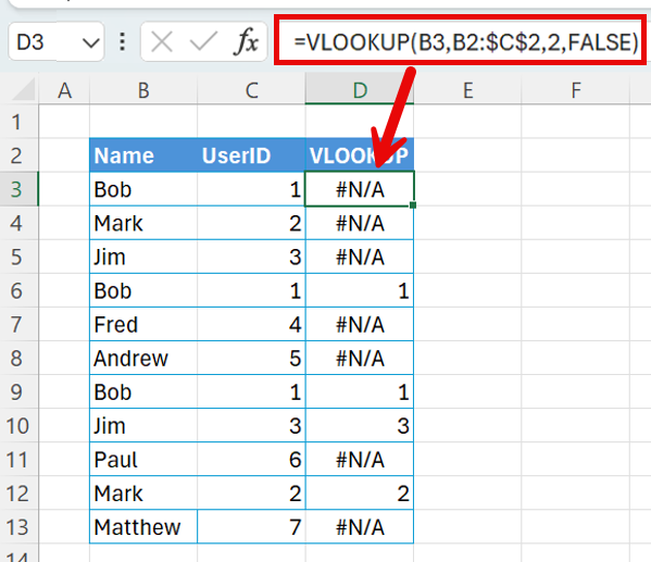
Therefore as the names Bob, Jim and Mark are repeated in the list, the VLOOKUP function will find the names and return the UserID that is associated with their name, otherwise it will return #N/A.

IF Function

We now join all these formulas together using the IF function.

=IF(ISNA(MATCH(B3,B2:$B$2,0)),MAX(C2:$C$2)+1,VLOOKUP(B3,B2:$C$2,2,FALSE))

IF ISNA function returns a TRUE for the MATCH function, then the TRUE part of the IF statement will run .  IF the ISNA function returns as FALSE for the MATCH function, the VLOOKUP Function will be used.

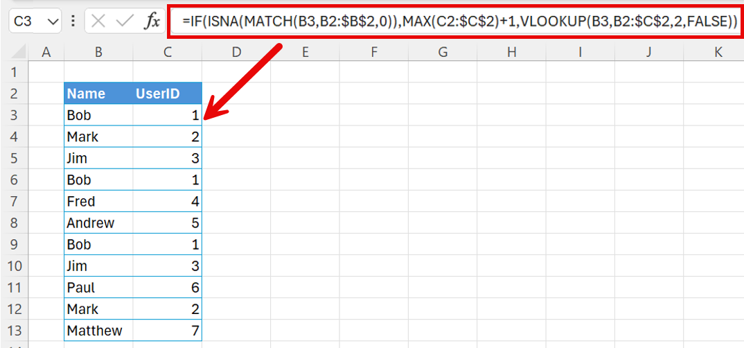
Due to the fact that we are using absolute reference in our formula, the formula changes as it is copied down through the rows – using the row above values to determine the output of the row that the formula is in.  This gives us the ability to create our unique ID’s.

Create Unique IDs in Google Sheets

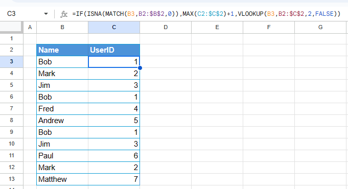
Google sheets uses the same formulas to create Unique ID’s