How to Sort Data in Excel & Google Sheets

This tutorial demonstrates how to sort data in Excel and Google Sheets.

 

Sort a Single Column of Text

1. Select any cell in the column of text you want to sort.

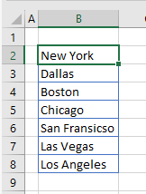
2. In the Ribbon, go to Data > Sort & Filter, and then click the A→Z sort button.

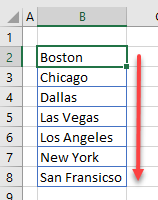
The column is sorted into alphabetical order, as shown below.

Sort Multiple Columns

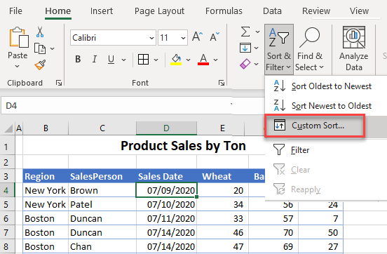
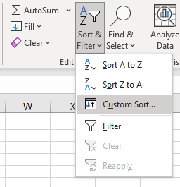
1. Make sure your cursor is position within the data table that you want to sort, and then in the Ribbon, go to Home > Editing > Sort & Filter > Custom Sort.

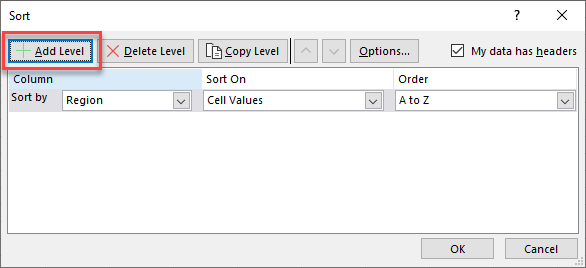
2. Choose a Column to Sort by, what to Sort On, and the Order you want to sort. Then click Add Level.

3. In the Then by drop down (below Sort by), choose a new column to sort. Continue to add each column you need.

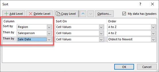
4. Click OK to sort.

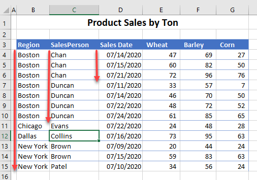
Tip: See How to Sort Multiple Columns for more information.

Sort by Custom List

It’s easy to sort alphabetically in Excel, but you can also sort by a more complex custom list.

1. Select the data you want to sort, and then in the Ribbon, go to Home > Editing > Sort & Filter > Custom Sort.
2. Choose the Column to Sort by and what to Sort On. Then in the Order drop down, choose Custom List…

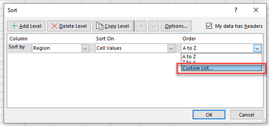
3. Select the custom list you want to sort by. If you don’t see the list you need, see How to Sort With a Custom List in Excel to learn how to create a new list.

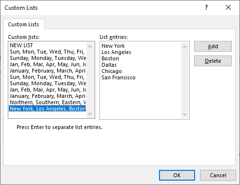
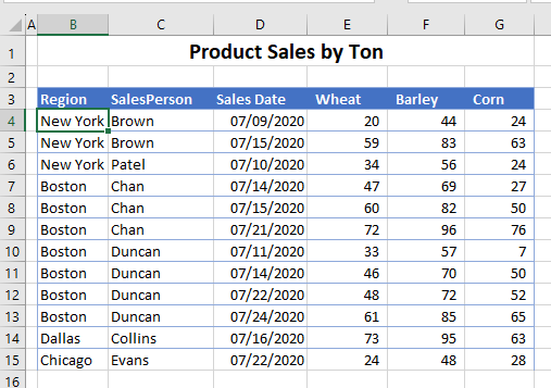
4. Click OK and then OK again to sort the data.

Sort Numbers

You can sort numbers from smallest to largest, or largest to smallest.

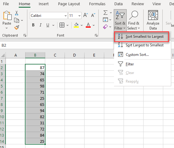
1. Select any cell in the column of numbers you want to sort.
2. In the Ribbon, go to Home > Editing > Sort & Filter > Sort Smallest to Largest.

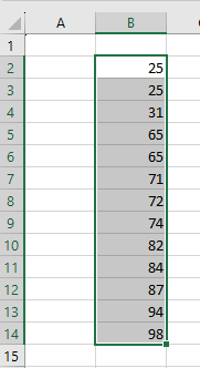
The numbers are then sorted.

Sort and Expand Selection

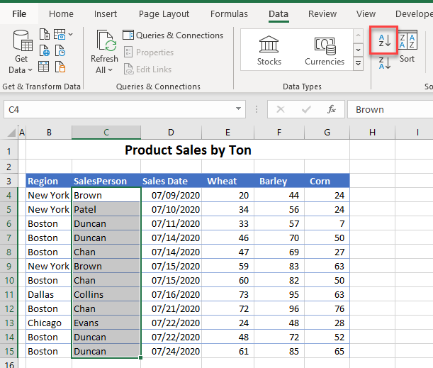
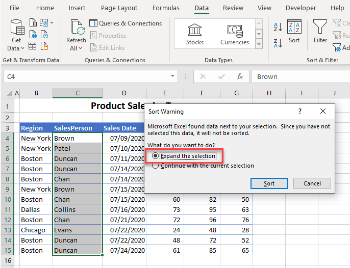
When your data is within a range of other data columns, Excel detects that you might need to expand the selection to sort out. If you do not do this, you end up sorting just the individual column and you may end up invalidating the data.

1. Select the column to sort in your data table.

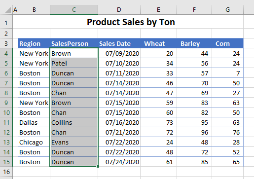
2. In the Ribbon, go to Data > Sort & Filter, and then click the A→Z sort button.

3. Choose Expand the selection, and then click Sort. This sorts all columns while keeping the rows together.

Sort Dates

1. Select any cell in a column of dates.

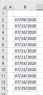
2. In the Ribbon, go to Home > Editing > Sort & Filter > Sort Oldest to Newest.

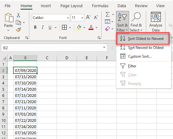
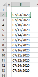
3. The rows are sorted with the row with the oldest date now being at the top of the data range.

Sort by Color

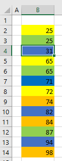
1. Select any cell in the table you want to sort.

2. In the Ribbon, go to Home > Editing > Sort & Filter > Custom Sort.

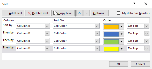
3. Choose any column to sort by, and then in the Sort On drop down, choose Cell Color.

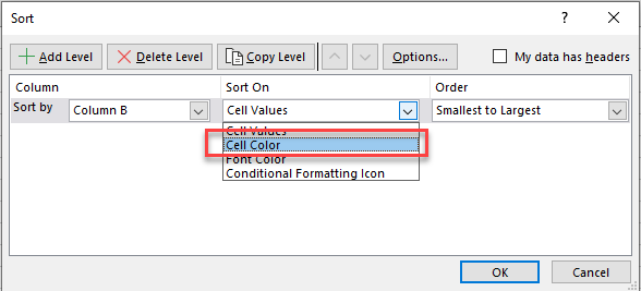
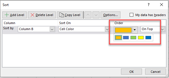
4. In the Order drop down, choose the color you want to display at the top of the sheet.

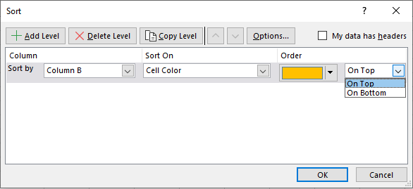
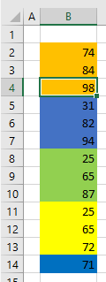
5. In the rightmost drop down, choose whether to sort the color at the beginning or end of the dataset. For this example, choose On Top, so orange rows are moved to the beginning.

6. Then click Add Level.

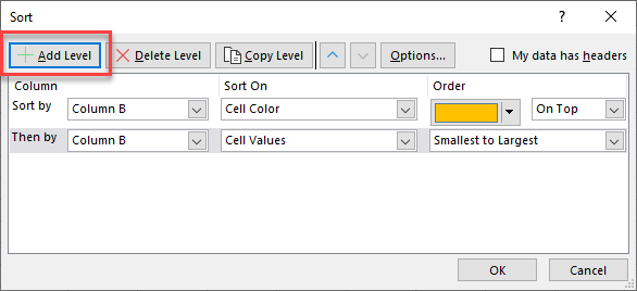
7. Use the same Column and leave Sort On as Cell Color. For Order, choose the color you want to display next and leave the last drop down as On Top. You can continue to add as many levels as you need.

8. Click OK to sort.

Horizonal Sort

You can also sort horizontally in Excel. If your field headings are set up as rows rather than columns, you don’t have to transpose the table to sort it.

1. Select the range to sort (here, C2:I7). Note that Column B (with the field headings) is excluded from the selection.

2. In the Ribbon, go to Home > Sort & Filter > Custom Sort.

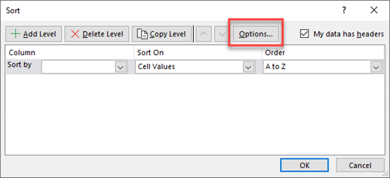
3. Click Options.

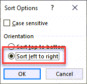
4. Choose Sort left to right, and click OK.

5. Choose a row to sort (e.g., Row 2 to sort by Salesperson). Leave the Sort On as Cell Values and the Order as A to Z, and then click OK.

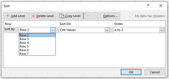
The data is then sorted from left to right based on the row chosen in Step 4.

Sort Filtered Data

If the data has a filter applied to it, each column has sort options available via filter buttons.

1. First, add a filter if there isn’t one already. In the Ribbon, go to Data > Sort & Filter > Filter.

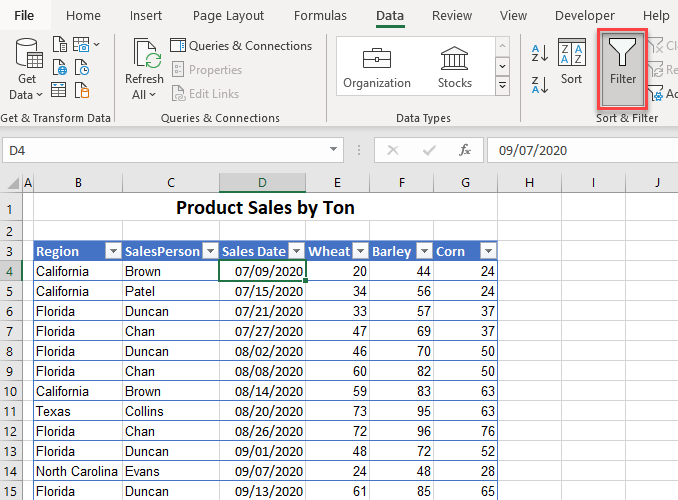
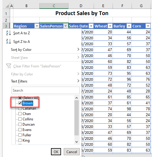
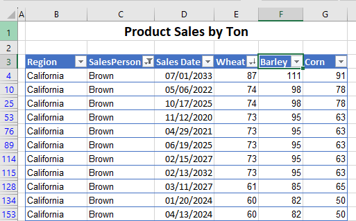
2. Notice a small arrow (filter button) at the top of each column of data. Click the arrow in the column of data you want to filter, and then tick the value to filter by (e.g., Salesperson Brown).

3. Select a different column to sort (e.g., Wheat) and this time, Sort Largest to Smallest.

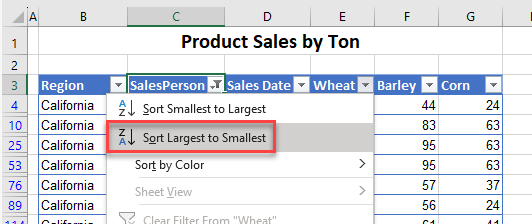
This sorts the filtered data.

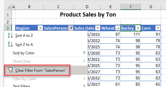
4. Select a cell back in the column that you filtered on and click Clear Filter From… in the filter drop down.

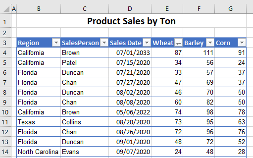
Notice that only the data that was visible during the filter was included in the sort.

Sort Table

Filtering as described above is also available when your data is formatted as a table.

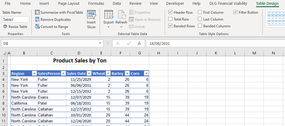
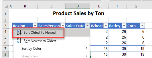
Click the filter arrow for the column you want to sort and choose:

• A→Z or Z→A for text columns;
• Oldest to Newest or Newest to Oldest for date columns; or
• Smallest to Largest or Largest to Smallest for number columns.

Sort Formulas

If you have a worksheet that constantly changes, you might need to re-sort the worksheet again and again with each change, since sorting is not dynamic. One way around this is to use a formula to automatically sort the data for you.

Consider the data below.

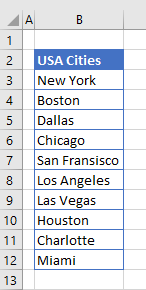
You could easily sort this data with Excel’s Sort feature, but preserve the data order in Column B with these steps:

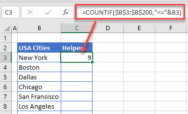
1. Insert a column to show how the data should be sorted. In this “helper” column, use the COUNTIF Function.

2. Copy the formula down to the other rows.

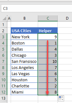
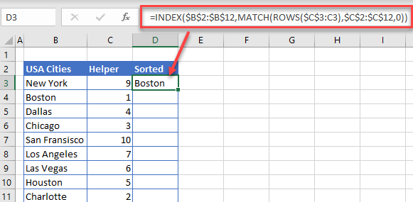
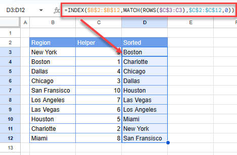
3. Then, use the next column for a formula containing the containing the INDEX, MATCH, and ROWS Functions to put the first column into alphabetical order.

   =INDEX($B$2:$B$12,MATCH(ROWS($C$3:C3),$C$2:$C$12,0))

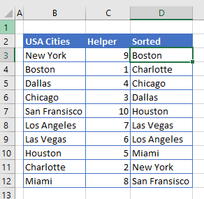
4. Copy the index–match formula down to the rest of the rows.

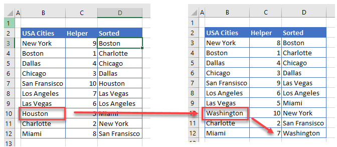
5. If you change one of the list items (e.g., Cities), then the sorted column automatically changes as well.

The SORT Function

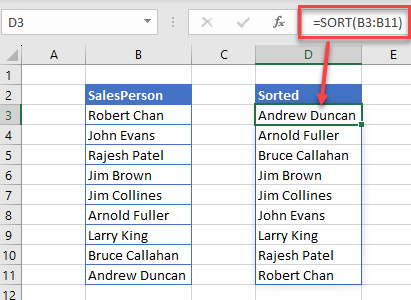
The SORT Function enables you to sort values in a range or an array.

Tip: You could use the SORT BY Function to achieve a similar result.

Sort and Ignore Blanks

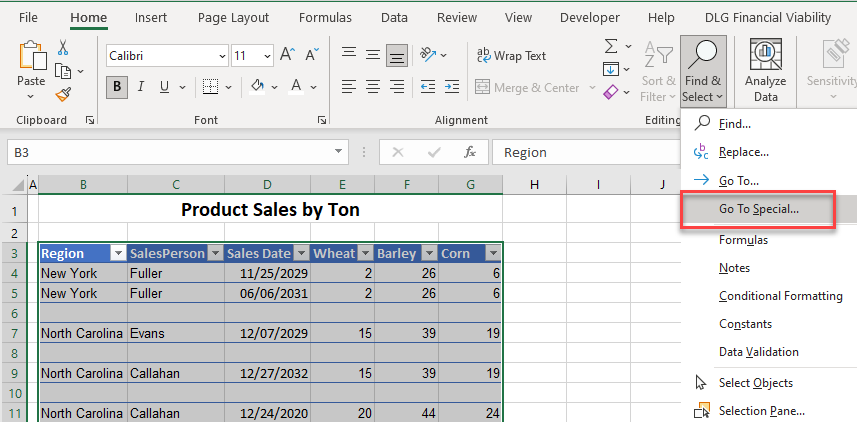
If you sort data that has blank rows in it, Excel pushes the blank rows to the bottom of the data. If you do not want the blank rows to be moved, you must hide the blank rows before you sort.

1. Highlight the data and then, in the Ribbon, go to Editing > Find & Select > Go To Special.

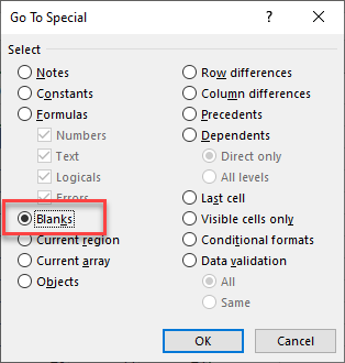
2. Choose Blanks, and then click OK.

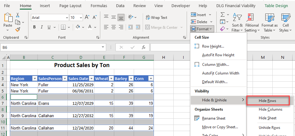
3. Now in the Ribbon, go to Cells > Forms > Hide & Unhide > Hide Rows.

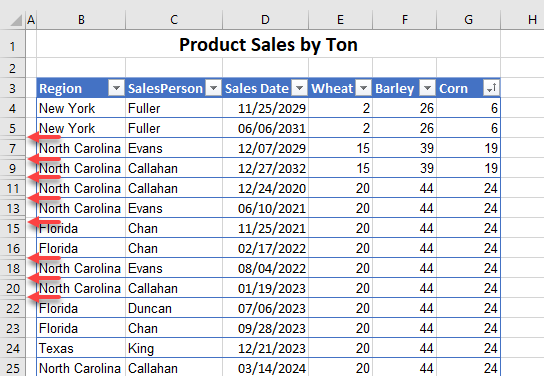
4. Then, select the column to sort and in the Ribbon, go to Home > Editing > Sort & Filter > Sort Smallest to Largest.
5. The data is then sorted in ascending order for the Corn column, but the hidden rows remain in place.

Sort Without Duplicates

If you have a list of numbers that you want to sort into ascending or descending order, but the list has a some duplicates in it, you can use formulas to sort the numbers while excluding the duplicates.

1. First, add a helper column containing the COUNTIF Function in the formula.

   =COUNTIF(B4:B$13,"="&B3)

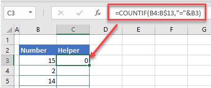
2. Copy the COUNTIF formula down to the remaining rows.

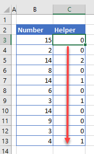
3. All unique numbers have a zero in their helper column, while duplicates have a positive or nonzero number.
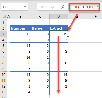
4. Write a simple IF statement to extract all the unique numbers, and then copy this formula down to the remaining rows.

   =IF(C3=0,B3,"")

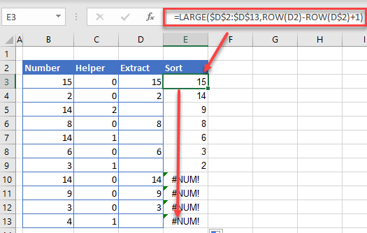
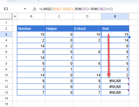
5. Finally, create another helper column to sort values from Column D without any blanks. Another formula can be used to achieve this using the LARGE and ROW Functions.

   =LARGE($D$2:$D$13,ROW(D2)-ROW(D$2)+1)

Issues That May Affect Sorting

For data to sort correctly, it needs to first be set up correctly. A few things to consider before sorting:

• Make sure there are no leading spaces in your data.
• Make sure that the column that you are sorting on contains the same type of data and not a mixture of text and numbers.
• It is useful to have a column heading for each column of data when sorting, then make sure that when you use Custom Sort, My data has headers is ticked.
• It is preferable to not have any blank rows or columns within your data.
• If your data contains formulas referencing the sheet name, you might need to remove the sheet name from the formula, if the reference is on the same sheet.

Sort With VBA

You can also use VBA code to sort. Here’s an example of a simple macro to sort by the first column on a range of data:

Sub SortMe()
  Worksheets("Sheet1").Sort.SortFields.Clear
  Range("B3:G100").Sort Key1:=Range("B3"), Header:=xlYes
End Sub

Sort in Google Sheets

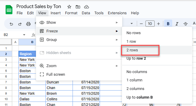
Google Sheets can’t automatically identify a header row in a dataset. To identify a header row, first freeze the row you want to use as the header.

Sort Sheet

1. Click in the row you want to freeze and then in the Menu, go to View > Freeze > 2 rows (or n rows, depending on your layout).

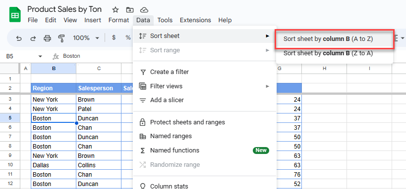
2. Then select any cell in the column you want to sort. In the Menu, go to Data > Sort sheet > Sort sheet by column…

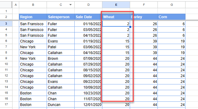
3. You can sort text, numbers, and dates by selecting the relevant column and going to Sort sheet.

Sort by Range

To sort by more than one column, you need to sort the data range.

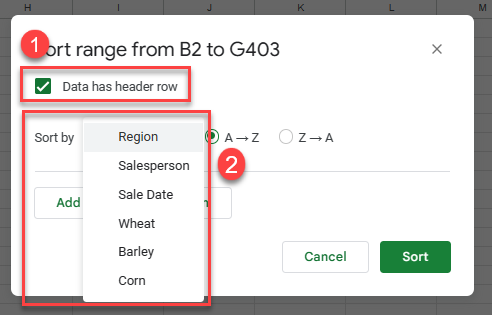
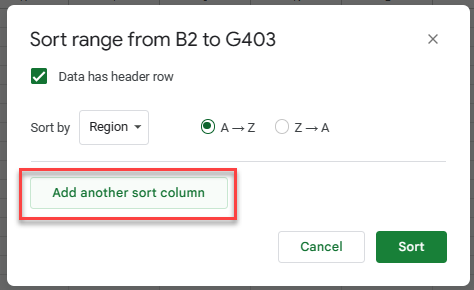
1. Select the sort range, and then in the Menu, go to Data > Sort range > Advanced range sorting options.

2. Check Data has header row, and then select the column to sort by. Choose A→Z to sort alphabetically or Z→A to sort in reverse order.

3. Click Add another sort column.

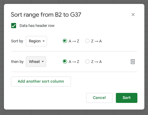
4. Select the next column you wish to sort by, and once again, choose A→Z or Z→A.

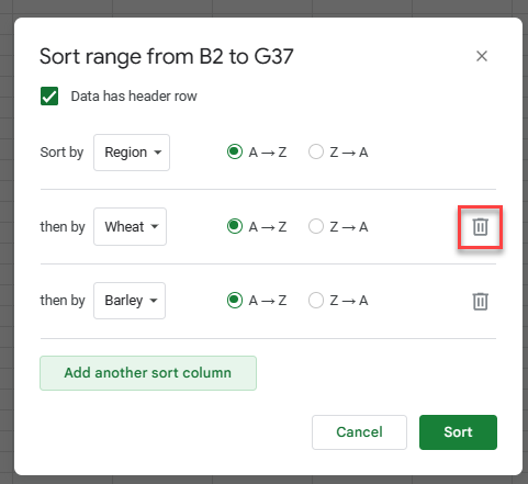
5. Continue to add as many columns as you need to your sort range. If you add one by mistake, click the Delete button to remove it from the sort.

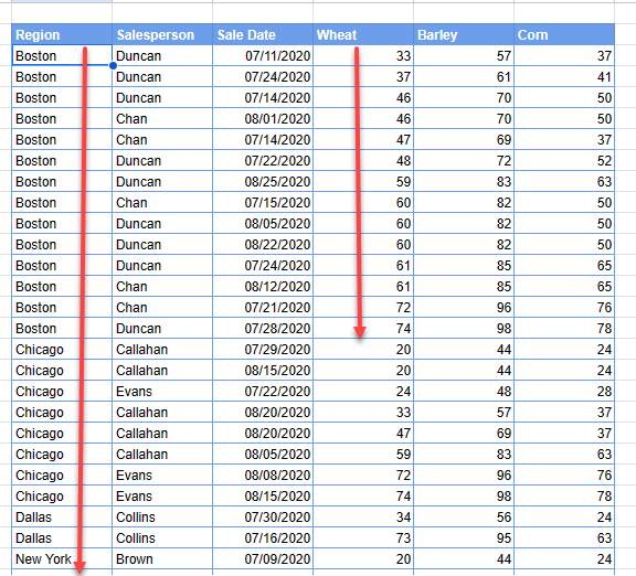
6. Click Sort to sort the data.

Sort Filtered Data

Sorting filtered data works the same in Google Sheets as it does in Excel.

1. First, add a filter. Click within your data and then, in the Menu, go to Data > Create a filter.

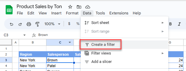
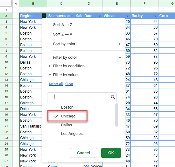
2. Then, filter on a selected column, for example, filter the Region column by the value Chicago.

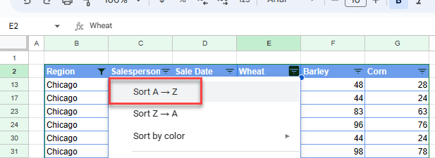
3. Sort A→Z on the Wheat column.
   (Google Sheets doesn’t differentiate between numbers and text for sort order options. Here, A→Z means lowest to highest.)

4. Remove the filter from Region; click the filter button, then Select all, then OK.

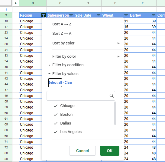
Note that the Wheat column in other regions (e.g., New York, Boston) is not sorted, but the Chicago Wheat numbers are sorted (in cells visible with the filter on).

Sort by Color

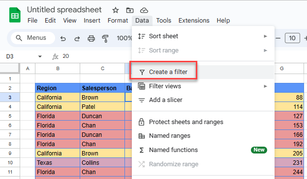
You can sort by color in Google Sheets, but you need to add a filter first.

1. Click within your data, and then in the Menu, go to Data > Create a filter.

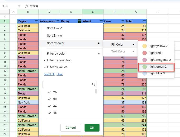
2. Then, click one of the column’s filter button. Go to Sort by color > Fill color, and then choose the color (e.g., light green 2) you want at the top of the table.

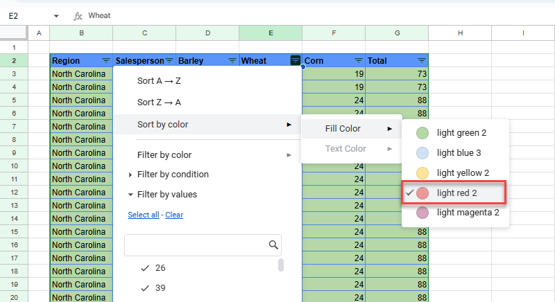
3. To sort by a second color, select a different column and repeat Step 2 for the second color (e.g., light red 2).

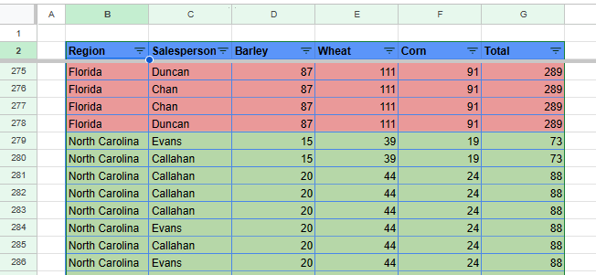
Rows with the second sort color (red) from Step 3 are sorted to the top of the table, and rows with the first sort color (green) from Step 2 are directly below the red rows.

Sort and Ignore Blanks

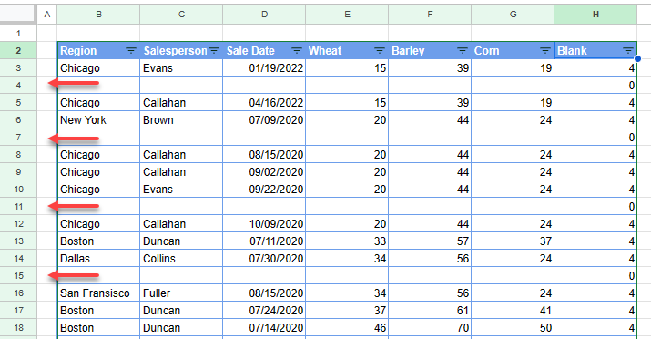
To ignore blank rows in Google Sheets, first add a helper column to filter out the blank rows.

1. In the column to the right of your data, enter a formula to count the number of populated cells in the selected row and copy the formula down to the rest of the rows in your data.

   =COUNT(B3:G3)

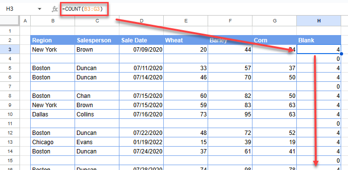
2. Then add a filter to your data, and filter the “blank” column to only show the rows where the cells are populated.

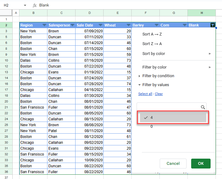
3. Now in a different column, choose Sort A→Z, and then click OK.

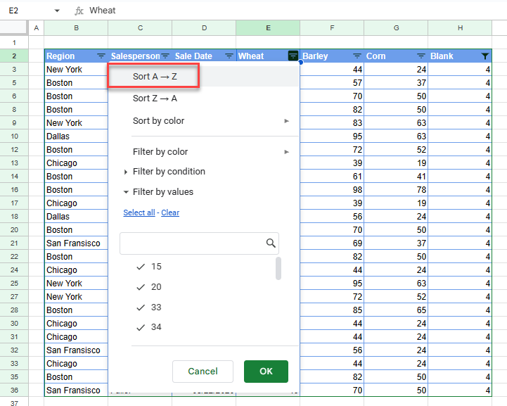
Only visible data gets sorted.

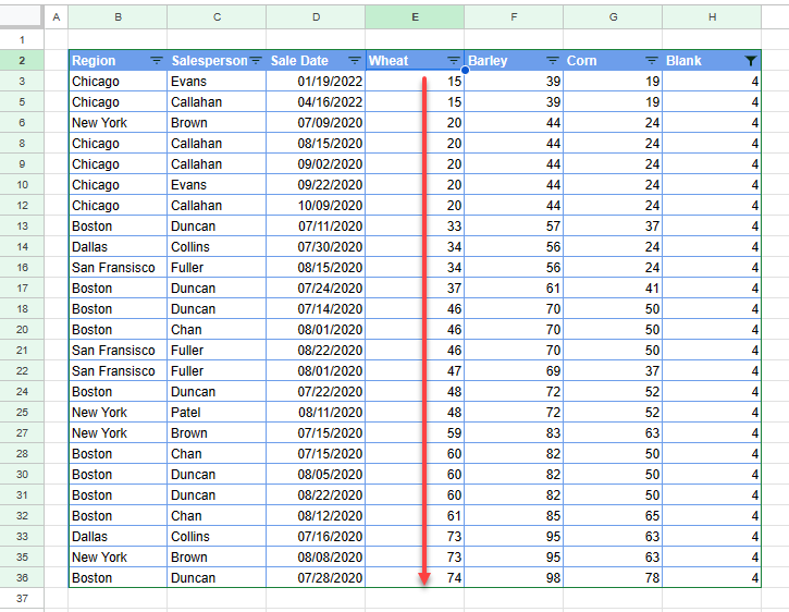
4. Remove the filter on the Blank column. Like in Excel, the blank (filtered out) rows haven’t moved.

Sort With Formulas

As you do in Excel, you can also use the COUNTIF, INDEX, MATCH, and ROWS Functions in formulas to sort in Google Sheets.

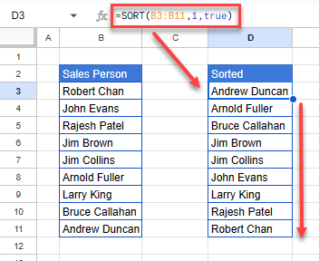
Or, use the SORT Function to sort in a column to the right of your original data.

You can sort duplicates using Formulas in the same way that you sort duplicates using formulas in Excel.

More Sort Tutorials

Read more of our tutorials on sorting in Excel and Google Sheets.

Sort Data
Advanced Sorting
Keep Rows Together During Sort
Put Things in Alphabetical Order
Random Sort
Reverse the Order of Data
Sort a Column Alphabetically
Sort and Ignore Blanks
Sort by Color (Highlighted Cells)
Sort by Last Name
Sort By Month
Sort By Number
Sort Dates in Chronological Order
Sort IP Addresses
Sort Multiple Columns
Sort Multiple Rows Horizontally
Sort Subtotals
Sort With a Custom List
Sort Without Duplicates
Undo a Sort
Calculation	yes
Keep Variable Cell Constant
Lock / Freeze Cell in Formula
Copy & Paste	yes
Copy Every Other Row
Database	yes
Clean Up Data
Create a Searchable Database
Drop-Down List	yes
Alphabetize a Drop Down-List
Duplicates	yes
Show Only Duplicates
Filters	yes
Apply Multiple Filters
Clear All Filters
Copy Filtered (Visible) Data
Filter by Color
Filter Merged Cells
Filter Rows
Hide Blank Rows
Hide Rows Based on Cell Value
Remove Filters
Show or Hide AutoFilter Arrows
Show Rows With Specific Text
Use Custom AutoFilters
Find & Select	yes
Select Every Other Row
Select Multiple Cells
Forecast	yes
Quick Analysis Tool
Format Cells	yes
Make All Rows and Columns the Same Height and Width
Formulas	yes
Custom Sort List with Formula
Sort Multiple Columns with Formula
Sort with SMALL & LARGE Functions
Functions	yes
SORT Function Examples
Insert & Delete	yes
Delete Blank Rows
Delete Every Other Column
Delete Every Other Row
Insert Blank Row After Every Other Row
Objects	yes
Make a Combo Box
Outline	yes
Expand or Collapse Rows or Columns
Text to Columns	yes
Split a Cell into Two or More Columns
VBA	yes
VBA Sort Array
Sorting Data in Excel VBA