How to Show Rows With Specific Text in Excel & Google Sheets

This tutorial demonstrates how to show rows containing specific text in Excel and Google Sheets.

 

 

Show Rows That Contain Specific Text

In Excel, you can use filters to show only some rows in a range. Say you have the following list of products in Column B and want to display rows only if they have specific text.

 

 

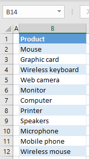
To show only rows that contain the word mouse, use a filter.

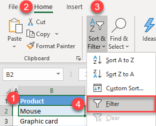
1. First, turn on the filter. Click on any cell in the range (B1:B12) and in the Ribbon, go to Home > Sort & Filter > Filter.

 

 

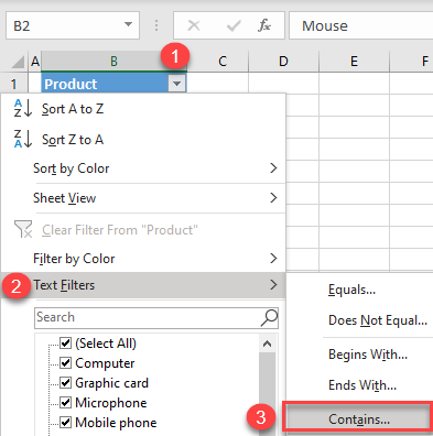
2. Click on the filter button next to Product (cell B1), go to Text Filters, and choose Contains…

 

 

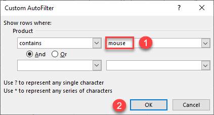
3. In the pop-up window, enter mouse in the field to the right of “contains,” and click OK.

 

 

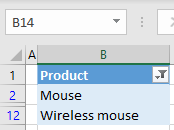
As a result, only cells containing –mouse– (cells B2 and B12) are displayed, while other cells are hidden. Note that Excel is not case-sensitive in filter conditions, so both uppercase and lowercase values are filtered.

 

 

Filter Text That Begins With

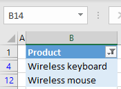
You can also show only rows that begin with wireless–.

1. Click on the filter button next to Product, choose Text Filters, and click Begins With…

 

 

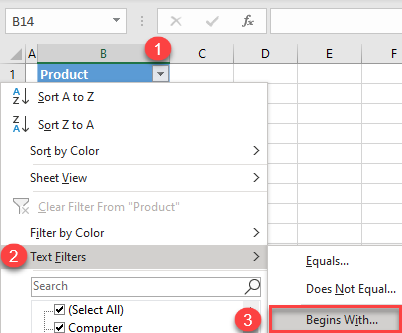
2. In the pop-up window, enter wireless in the field to the right of “begins with,” and click OK.

 

 

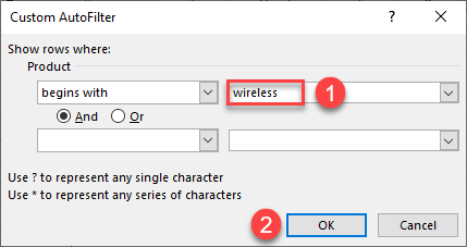
As a result, only cells beginning with wireless– (cells B4 and B12) are displayed; all other cells are hidden.

 

 

Filter Text That Ends With

Another possibility is to show only rows that end with –phone.

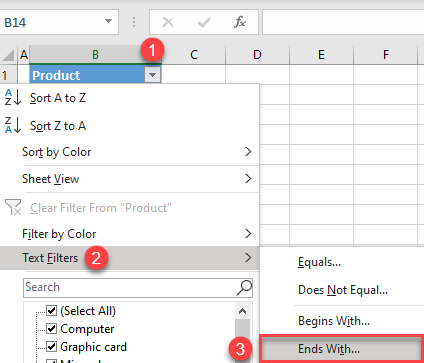
1. Click on the filter button next to Product, choose Text Filters, and click Ends With…

 

 

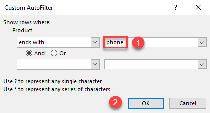
2. In the pop-up window, enter phone in the field to the right of “ends with,” and click OK.

 

 

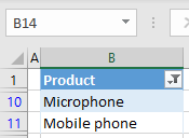
As a result, only cells ending with –phone (cells B10 and B11) are displayed; all other cells are hidden.

 

 

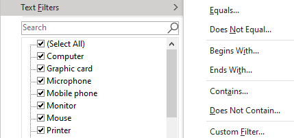
Other options for filtering using text filter include:

• equals / does not equal,
• does not contain, and
• custom filter.

Show Rows That Contain Specific Text in Google Sheets

In Google Sheets, you can filter rows based on text in almost the same way. Let’s use the same example to display rows containing –mouse– in Column B.

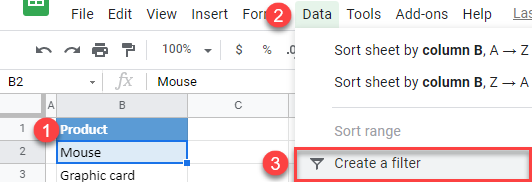
1. First, create a filter by clicking anywhere in the data range (B2:B12) and in the Menu, going to Data > Create a filter.

 

 

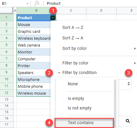
2. Click on the filter button next to Product (cell B2) and go to Filter by condition. In the drop-down list, choose Text contains.

 

 

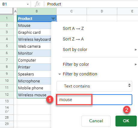
3. Enter mouse in the text box and click OK.

 

 

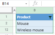
As a result, only rows with the text –mouse– in Column B are displayed.

 

 

Like Excel, Google Sheets has more options to filter by text:

• text does not contain,
• text starts/ends with,
• text is exactly, and
• custom formula.