How to Remove Both Duplicates (Rows) in Excel & Google Sheets
Written by
Reviewed by
This tutorial demonstrates how to identify duplicate rows and remove both of them in Excel and Google Sheets.
Remove Both Duplicate Rows
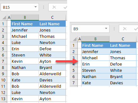
Generally, when you remove duplicates in Excel, the first occurrence of each duplicate is kept, and all others are deleted.
Another valuable task is to remove both (or all) duplicate rows. This can be achieved using a combination of the IF and COUNTIF Functions and the Go To Special feature. See the example data below. Columns B and C have a list of first and last names containing duplicate values.
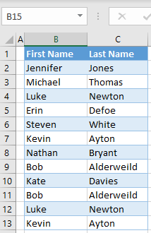
Follow these steps to remove all duplicate rows and keep only those with unique values:
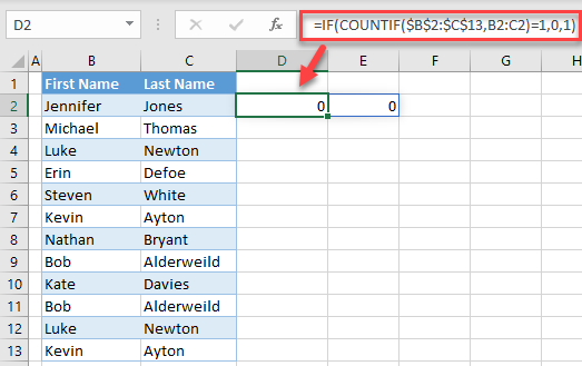
- In cell D2, enter the formula:
=IF(COUNTIF($B$2:$C$13,B2:C2)=1,0,1)The COUNTIF Function checks for every cell if it is in some other cell in a range. The IF Function only checks the result of the COUNTIF. If the COUNTIF returns one that means that the value is unique in the range, while all other number means that the value is appearing more than once. Therefore, the final result of the formula is zero if the COUNTIF returns one, and one if it returns anything else. This formula outputs two values (in D2 and E2), one for each First Name and one for each Last Name.
- Position the cursor in the bottom-right corner of cell D2 until the black cross appears and drag it through the end of the data range (D13).
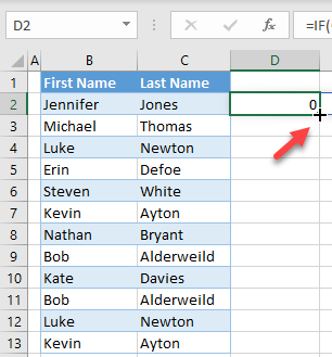
- As a result of Step 2, there is a zero or a one in Columns D and E for each value in Columns B and C. A zero means that a value from Columns B or C is not repeating in the data range and should be kept. A one means that there are duplicate values and that row should be deleted.
Now, click anywhere in Column B with data (B2), and in the Ribbon, go to Data > Filter.
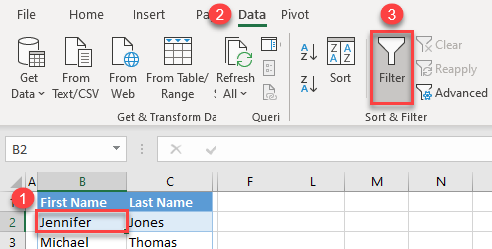
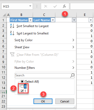
- Now filters are turned on. To delete duplicate rows, filter out zeros from Columns B and C. Since duplicates have ones in both Columns D and E, display and delete only values with ones in Columns D and E.
Click on the filter button in Column D, uncheck 0, and click OK.
- Now check the filter for Column E to be sure that only the value 1 is filtered.
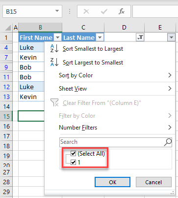
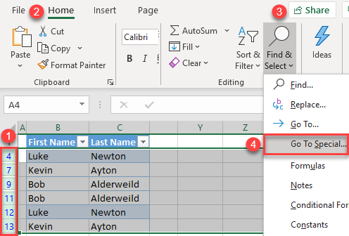
- To delete all filtered rows, select all visible rows (4–13), and in the Ribbon, go to Home > Find & Select > Go To Special.
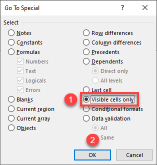
- In the Go To Special window, select Visible cells only, and click OK.
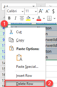
- Now delete only visible rows. Select all filtered cells (4–13) and right-click anywhere in the selected area. Then click Delete Row.
- Now, click on the filter button in cell D1 and click Select All (0).
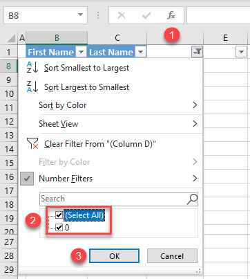
Finally, the data range is filtered by Column D (0 values).
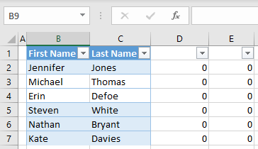
All rows with zeros in Columns D and E are unique values in the range; rows with ones in those columns (duplicate values) are deleted.
You can also use VBA code to remove duplicate rows in Excel.
Remove Both Duplicate Rows in Google Sheets
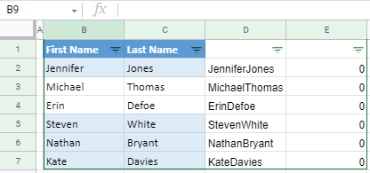
In Google Sheets, you can also delete all duplicate rows using the IF and COUNTIF Functions.
- First, create a helper column (Column D) to concatenate text from Columns B and C. In the cell D2, enter the formula:
=CONCATENATE(B2:C2)
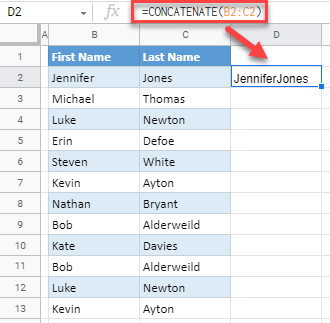
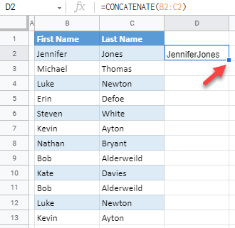
- Position the cursor in the bottom-right corner of cell D2 until the black cross appears and drag it through the end of the data range (D13).
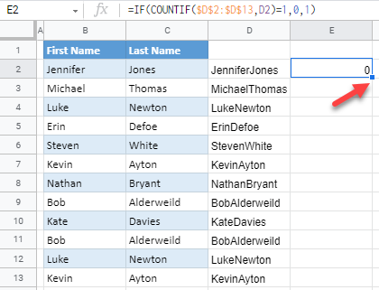
- In cell E2, enter the formula:
=IF(COUNTIF($D$2:$D$13,D2)=1,0,1)This is similar to the formula shown for Excel in the section above, but instead of looking at first and last names separately, it looks at the concatenated name in Column D.
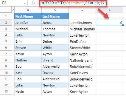
- Position the cursor in the bottom-right corner of cell E2 until the black cross appears and drag it through the end of the data range (E13).
- Select a cell in Column E (E2) and click on the Filter icon in the toolbar to turn on filters.

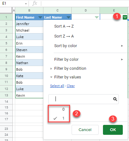
- Click the filter icon for Column E (cell E1), uncheck 0, and click OK.
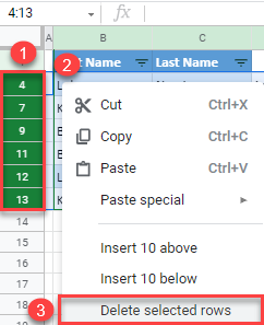
- Select and right-click filtered rows. Then click Delete selected rows. In Google Sheets, there’s nothing like Excel’s Go To Special feature. Google Sheets always deletes only visible rows.
- Click on the filter icon for Column E (E1), check 0, and click OK.
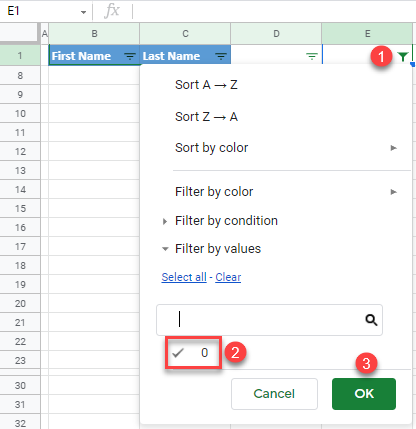
As a result, only unique rows (with 0 in Column E) are displayed.
