Pivot Table Sorting Guide (New for 2023!) Excel & Google Sheets

This tutorial demonstrates various ways to sort data in a pivot table in Excel and Google Sheets.

 

 

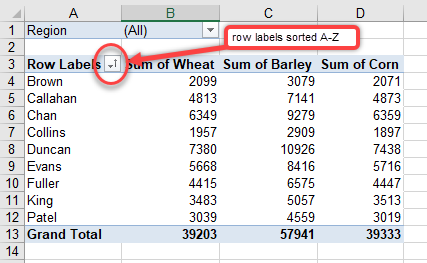
When you create a pivot table, you may wish to arrange the data – in alphabetical order for text fields or numerical order for value fields. You can sort both labels and fields within a pivot table by using drop-down filter buttons within the pivot table, or by using Sort through the Ribbon.

Sort by Row Labels

Consider the pivot table below.

 

 

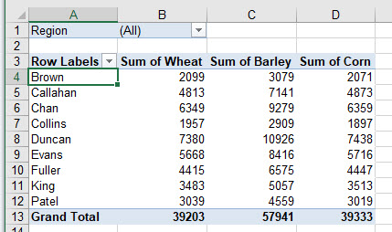
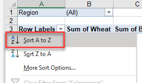
1. To sort the row labels from A–Z (ascending alphabetical order), first click anywhere in the list under the Row Labels heading.

 

 

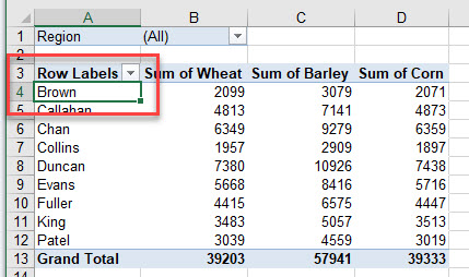
2. Then in the Ribbon, go to Home > Editing > Sort & Filter > Sort A to Z.

 

 

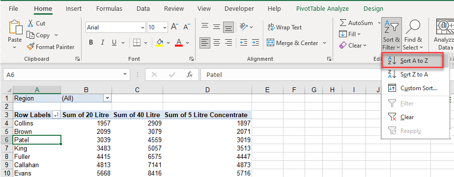
3. Click Sort A to Z.

 

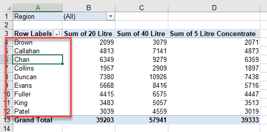
The row items are sorted in alphabetical order.

 

 

You can, of course, also use Z to A and sort in the reverse order.

More Sort Options

1. For more sorting options, click the arrow on the right side of the Row Labels cell, and then choose More Sort Options…

 

 

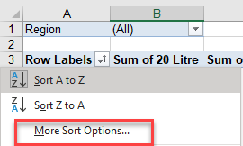
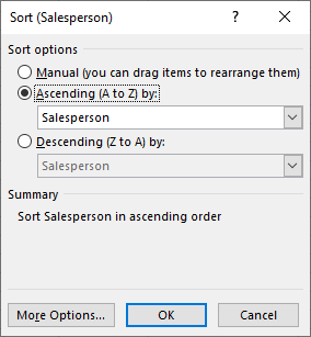
2. This brings up the Sort options dialog box where you can choose to sort Manually, Ascending, or Descending.

 

 

Manual Sort

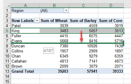
1. Click Manual, and then click OK.
2. Then drag individual rows of data up or down on the pivot table.

 

 

Ascending / Descending

1. From within the Sort options dialog box, use Ascending or Descending. While this is the same as sorting A–Z or Z–A as described previously, it lets you choose the field to sort by.

 

 

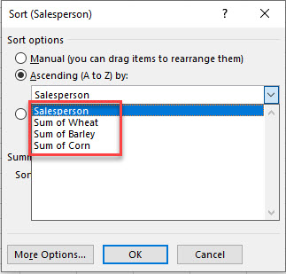
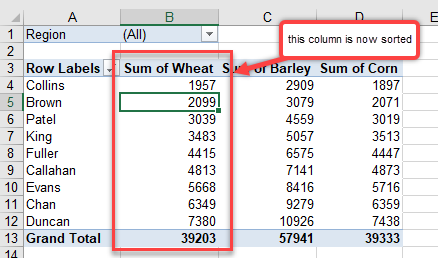
2. For example, choose Wheat instead of Salesperson.

 

 

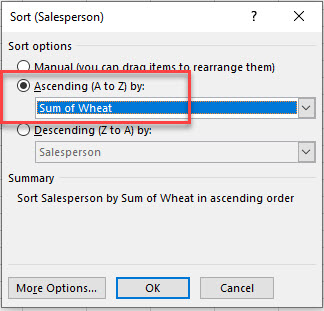
Since Wheat is a value column, it’s sorted from smallest to largest rather than from A–Z.

 

 

Custom List

1. While in the Sort options dialog box, click More Options…

 

 

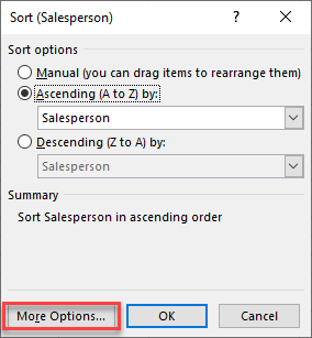
2. Leave AutoSort (Sort automatically every time the report is updated) checked.

 

 

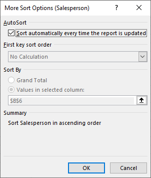
3. To sort by a specific list, uncheck AutoSort and choose another list from the First key sort order drop down.

 

 

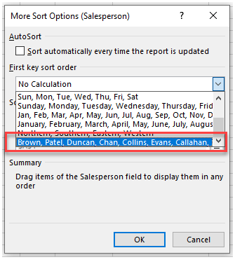
4. Click OK, and then OK again, to sort by your custom list.

Sort by Field Values

You can also choose to sort by a field’s values.

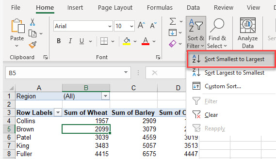
1. Click in the column of the field whose values you wish to sort (e.g., Wheat).
2. In the Ribbon, go to Home > Editing > Sort & Filter > Sort Smallest to Largest.

 

 

Sort Directions

1. In the Ribbon, go to Home > Editing > Sort & Filter > Custom Sort…

 

 

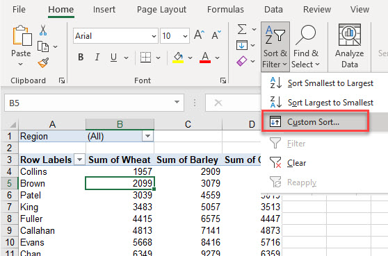
2. With Custom Sort, in addition to sorting from smallest to largest or largest to smallest, you can also sort from top to bottom or left to right.

 

 

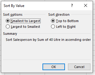
3. Choose Left to Right, and then click OK.

 

 

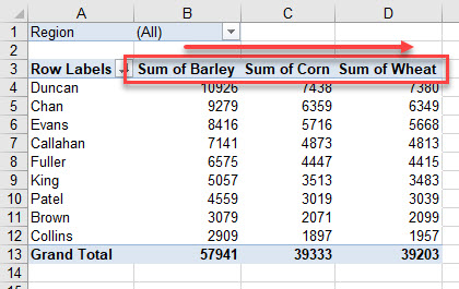
The result is the columns of the value fields arranged into alphabetical order from left to right.

Sort Order – Add New Data

If you add new data to the bottom of your source data, you many need to change the source data for your pivot table to make sure everything is included. But when you go to choose an item from the filter drop down, the list is not necessarily in alphabetical order anymore.

 

 

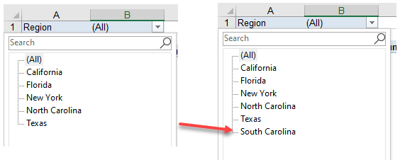
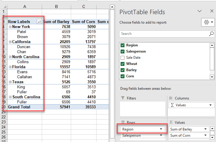
1. To correct the sort order, drag the field down from the Filters area to the Rows area.

 

 

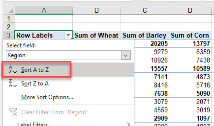
2. Then click on the field (e.g., Region) and sort from A to Z.

 

 

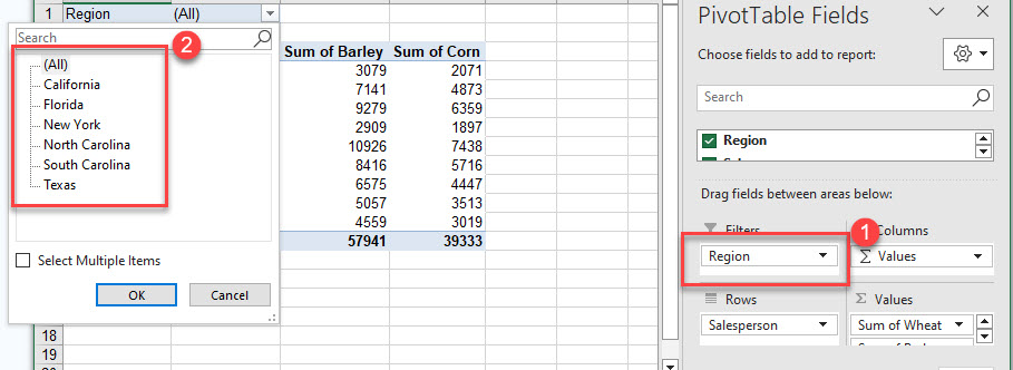
3. Next, move the field back to the Filters area from the Rows area. The list of items is then back in alphabetical order.

 

 

Sort Multiple Row Fields

You can add multiple row fields to a pivot table. The example below has both Region and Salesperson added as row fields.

 

 

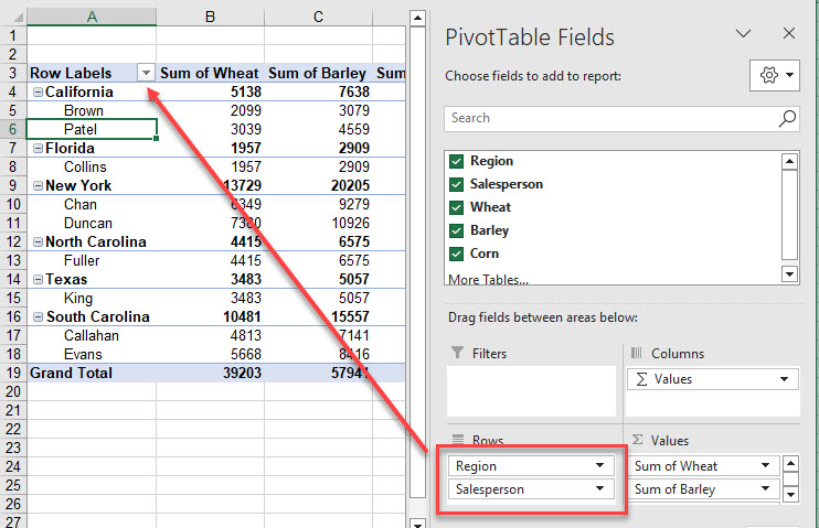
1. If you click in the Region field and click Sort A to Z, it sorts the regions in alphabetical order, but the names within each region may not be.
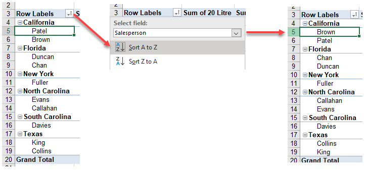
2. Click within the nested field (e.g., Salesperson), and then click Sort A to Z.

 

 

Tip: Try using some shortcuts when you’re working with pivot tables.

Sort Pivot Tables in Google Sheets

In Google Sheets, you can sort pivot tables by fields in the row or column or by values.

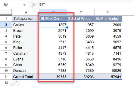
Consider the pivot table below.

 

 

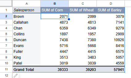
1. In the Pivot table editor to the right, in the Rows section, choose the field you want to sort by. By default, the table is sorted alphabetically (or numerically) by the row field, e.g., Salesperson.

 

 

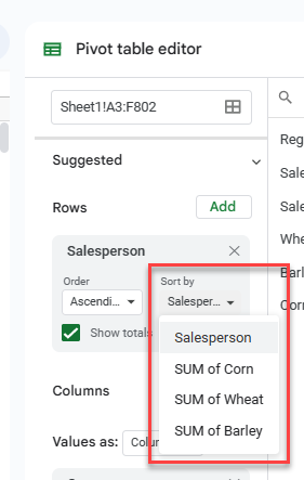
2. Choose a different field to sort by (e.g., Corn). Note that the values in your pivot table in the Corn column are now sorted from smallest to largest.