How to Create a Lookup Table in Excel & Google Sheets

This tutorial demonstrates how to create a lookup table in Excel and Google Sheets.

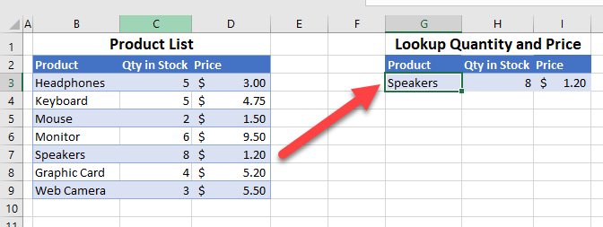
Table Source Data

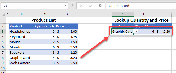
Say you have a table like the one below.

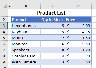
The data is set up as a searchable database, with the data is stored in columns – called field names, and in rows – called records. Each row holds the data for an individual Product. Setting out information in Excel in such a way enables you to sort and filter on the data, as well as use functions such as VLOOKUP. Your database can contain as many columns and rows available in a single Excel sheet (16,384 columns and 1,048,576 rows are available in each sheet but that might be a bit large for Excel to cope with!)

VLOOKUP Tables

A lookup table enables you to fetch data from your existing table or range of data using the VLOOKUP Function.

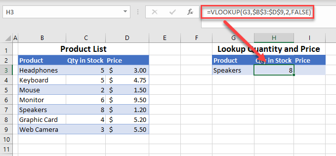
1. In cell G3, type in the name of the Product to look up the Qty in Stock and Price for.

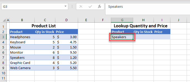
2. In cell H3, type in a VLOOKUP formula to get the Qty in Stock for that Product. Type the formula:

   =VLOOKUP(G3,$B$3:$D$9,2,FALSE)

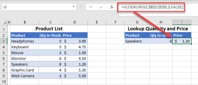
3. Repeat the process to look up the Price of the Product.

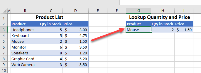
4. When you type in a different Product, the values in H3 and I3 change accordingly.

Drop-Down List

You can also create a drop-down list with data validation to choose a Product from a list instead of typing in the product’s name.

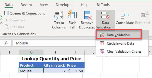
1. Click in the cell where you wish to insert the drop-down list, and then, in the Ribbon, go to Data > Data Tools > Data Validation > Data Validation.

2. You can then choose List and select the range for the drop-down list. You can also customize the input message and error alert if you wish.

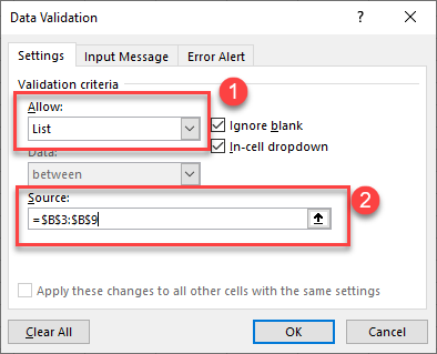
3. Click OK to create the drop-down list.

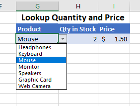
4. Choose a different Product from the list to look up the Qty and Price from the original table data.

Lookup Table in Google Sheets

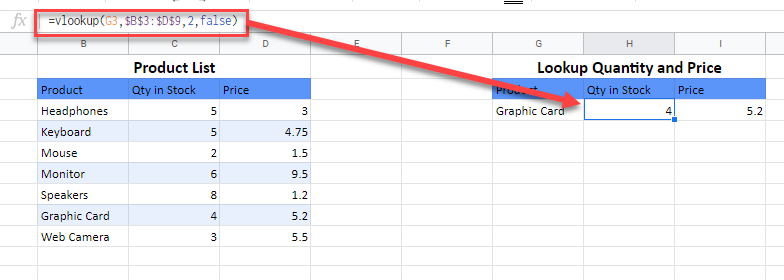
You can use the VLOOKUP Function to look up values in your table in Google Sheets as you do in Excel, with or without a drop-down list data validation cell.