How to Insert Blank Every Other Row in Excel & Google Sheets

This tutorial demonstrates how to insert a blank row after every other row in Excel and Google Sheets.

 

 

Insert Every Other Row with AutoMacro

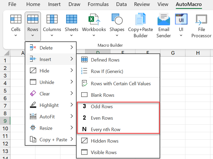
The easiest way to insert every other row in Excel is with AutoMacro for Excel. With a few clicks you can:

• Insert every other row – odd rows
• Insert every other row – even rows
• Insert every nth row
• Insert the rows once, or add a button to insert rows whenever you need it.

Learn More!

Insert a Blank Every Other Row

To insert a blank every other row (or every 3^rd, 4^th, or n^th row), follow these steps:

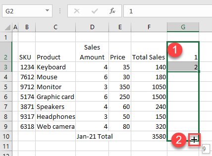
1. First, create a helper column. Enter 1 and 2 in the first two cells (G2 and G3), then drag down the fill handle to the last cell (G10).

 

 

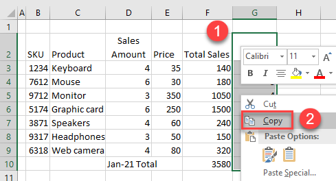
2. After you’ve filled the helper column with numbers, select all of them, right-click the selection, and choose Copy (or use the CTRL + C shortcut).

 

 

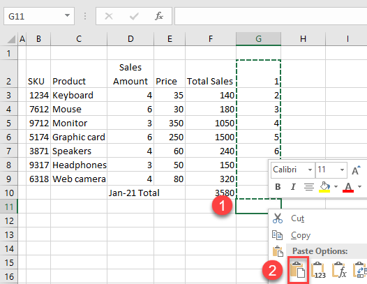
3. To paste the range, select the first empty cell in the helper column (G11), right-click it, and choose Paste (or use the CTRL + V shortcut).

Note: If you want to insert two or more blank rows between existing rows just copy and paste the helper column list two or more times below the last cell.

 

 

4. Now, select the data from the helper column and in the Ribbon, go to Home > Sort & Filter > Sort Smallest to Largest.

 

 

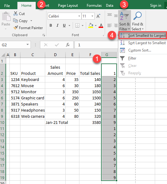
5. In the Sort Warning window, press Sort.

 

 

As a result, a space between each row appears.

 

 

6. To delete the helper column, select the data, right-click it, and choose Delete.

 

 

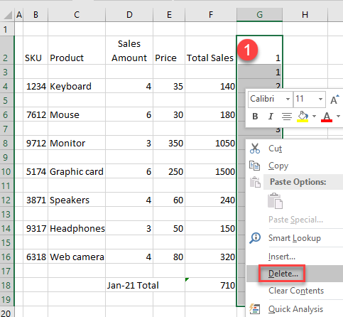
As a result, you get alternating data rows and blanks.

 

 

See also: VBA Insert Row or Column.

Insert Blank Every Other Row in Google Sheets

1. To insert blank every other row in Google Sheets, first create a helper column. In the helper column, enter 1 and 2 in the starting cells (F1 and F2). Drag down the fill handle to the last cell (F9).

 

 

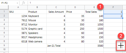
2. Select all numbers in the helper column, right-click them, and choose Copy (or use the CTRL + C shortcut).

 

 

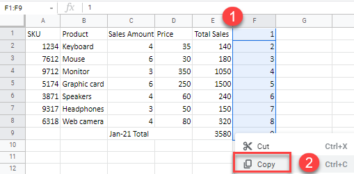
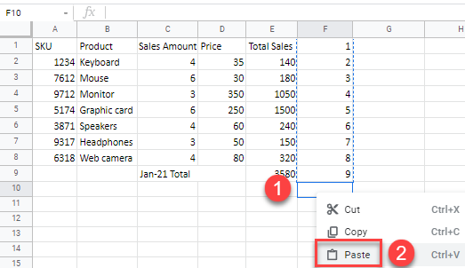
3. Then, select the first empty cell in the helper column (F10), right-click it (2), and choose Paste (or use the CTRL + V shortcut).

 

 

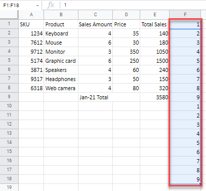
4. Select all data in the helper column (F1:F18).

 

 

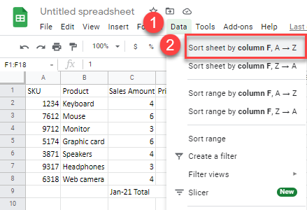
5. In the Menu, go to Data > Sort sheet by column F, A → Z.

 

 

As a result, blank rows appear between the existing ones. Now, you just need to delete the helper column.

 

 

6. To delete the helper column, select the data from the column, right-click it, and choose the Delete column.

 

 

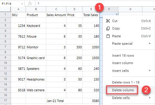
Now, you have alternating data rows and blanks.

 

 

You can always delete the blank rows later to make the worksheet more compatible with calculations.