Highlight Cell if Value Exists in Another Column in Excel & Google Sheets

This tutorial demonstrates how to highlight a cell if its value exists in another column in Excel and Google Sheets.

 

 

Highlight Cell if Value Exists in Another Column

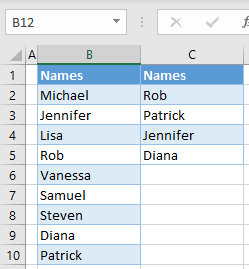
In Excel, you can use conditional formatting to highlight a cell if its value exists in another column. For this example, there is one list of names in Column B and another in Column C, as shown below.

 

 

Say you want to highlight in green all cells from Column B, which also exist in Column C.

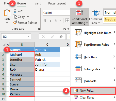
1. Select the data range to be highlighted and in the Ribbon, go to Home > Conditional Formatting > New Rule.

 

 

2. In the New Formatting Rule window, (1) select Use a formula to determine which cells to format for the Rule type and (2) enter the formula:

=NOT(ISERROR(VLOOKUP($B2,$C$2:$C$5,1,FALSE)))

Then (3) click Format.

 

 

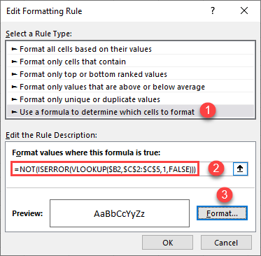
• The VLOOKUP Formula looks for a value from Column B in the range C2:C5.
• If the value is found, the ISERROR Function will return FALSE, because there is no error.
• The NOT Function will revert the result of the ISERROR Function, so FALSE becomes TRUE.

The formatting rule is applied only to the cells where the result of the formula is true.

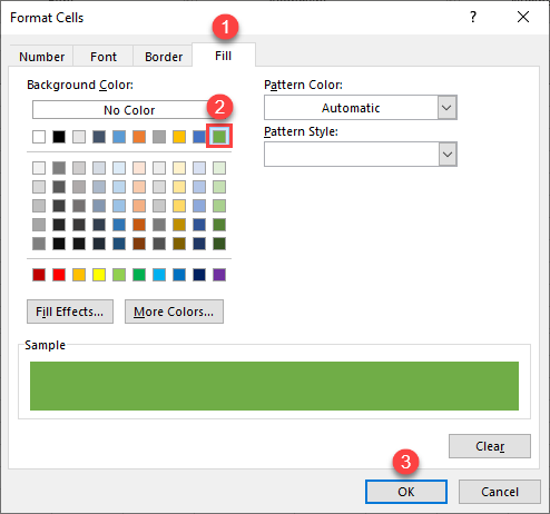
3. In the Format Cells window, go to the Fill tab, select a color (e.g., green) and click OK.

 

 

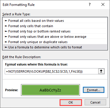
4. Now, you are back in the New Formatting Rule window, where you can see a preview of the formatting. Click OK.

 

 

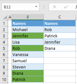
As a result, cells from Column B that also exist in Column C (B3, B5, B9, and B10) are highlighted in green.

 

 

Highlight a Cell if Its Value Exists in Another Column in Google Sheets

You can use the same in Google Sheets as is shown above in Excel.

1. Select the data range to be highlighted (B2:B10), and in the Ribbon, go to Format > Conditional formatting.

 

 

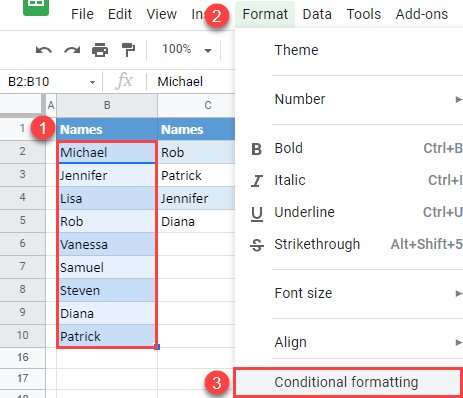
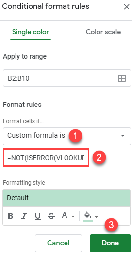
2. In the Conditional Format rules window on the right side, (1) choose Custom formula is from the Format rules drop down and (2) enter the formula:

=NOT(ISERROR(VLOOKUP($B2,$C$2:$C$5,1,FALSE)))

Then (3) Click Done, leaving green as the highlight color in the cell. This can be changed later by clicking on the fill color icon.

 

 

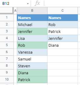
Finally, all cells from Column B that also exist in Column C are highlighted.