How to Hide / Suppress Zeros in Excel & Google Sheets

In this tutorial, you will learn how to hide zeros in Excel and Google Sheets.

 

 

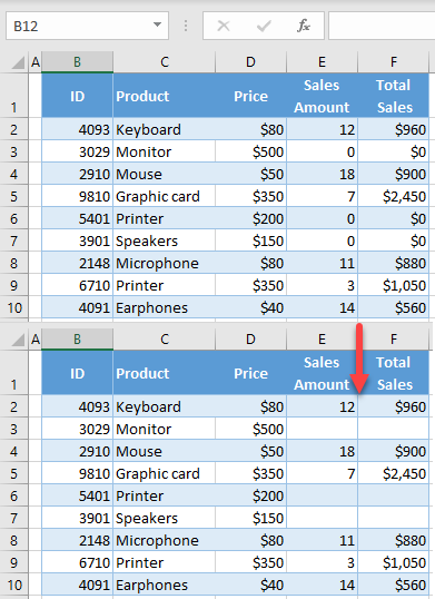
There are several ways to hide zero values in Excel:

• Hide zeros in the whole workbook using Excel Options.
• Hide zeros using a custom number format.
• Hide zeros with conditional formatting.

Hide Zeros – Excel Options

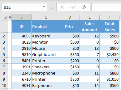
In the Excel Options, you can disable showing zeros for zero values for a worksheet or for a whole workbook. In this case, cells with zero values will be empty. Say you have the following data set with zero values in several cells.

 

 

To make zero cells empty, follow these steps:

1. In the Ribbon go to File > Options.

 

 

2. In the Excel Options window, go to Advanced, scroll down to the Display options, uncheck Show a zero in cells that have zero value, and click OK.

 

 

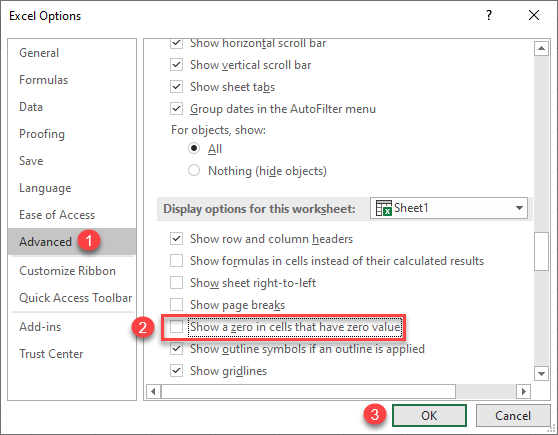
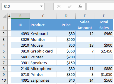
As a result, all cells with zero values are now empty.

 

 

Hide Zeros With a Custom Number Format

Another option to suppress zeros is to use a custom number format.

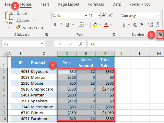
1. Select a range of cells with zero values, go to the Home tab, and click on the Number format icon in the right lower corner of the Number group.

 

 

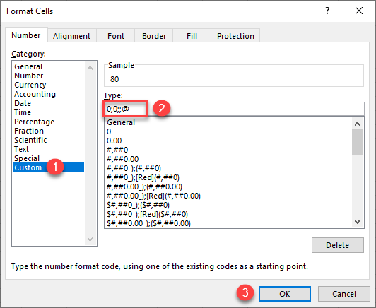
2. In the Format Cells window, (1) go to the Custom category, (2) enter 0;0;;@ for Type, and (3) press OK.
   If you have values with currencies, enter the currency first ($0;0;;@). Use this format for Columns D and F in our case.

 

 

The result is the same as above with (Excel Options): All zeros are suppressed and displayed as empty cells.

 

 

Hide Zeros With Conditional Formatting

A third option to hide zeros in a worksheet is to use conditional formatting. As a prerequisite for this method, all cells with zero values must have the same background color, so you can set the conditional formatting font color to the background color (in this case, white).

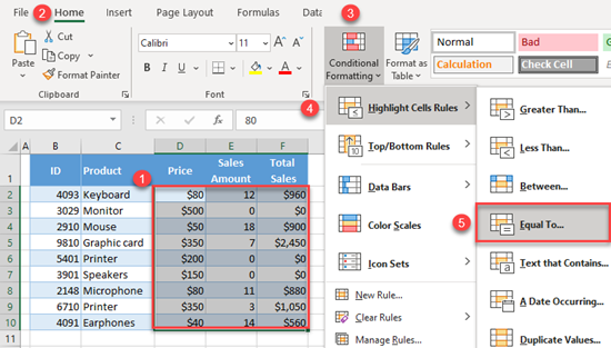
1. Select a range of cells that you want to format (e.g., D2:F10), and in the Ribbon, go to Home > Conditional Formatting > Highlight Cells Rules > Equal To.

 

 

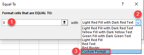
2. In the pop-up window, enter 0 in the left box, and choose Custom Format from the drop-down menu on the right.

 

 

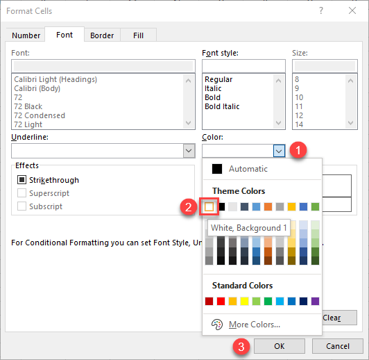
3. In the Format Cells window, click on the Color drop-down menu, choose white, and press OK.

 

 

The result is again the same: All zero values are suppressed.

 

 

Hide Zeros With a Custom Number Format in Google Sheets

To hide zeros by setting and applying a custom number format in Google Sheets, follow these steps:

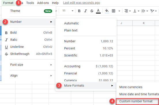
1. Select a range of cells with zero values (D2:F10), and go to Format > Number > More Formats > Custom number format.

 

 

2. In the Custom number formats window, enter 0;0;;@, and press Apply.
   For values with currencies, enter the currency first ($0;0;;@). Use this for Columns D and F in this example.

 

 

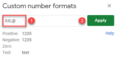
The result is the same as in Excel: All zeros are suppressed and displayed as empty cells.

 

 

Hide Zeros With Conditional Formatting in Google Sheets

Just like in Excel, the background cell color needs to be uniform to create conditional formatting that suppresses zero values in Google Sheets.

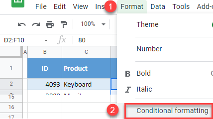
1. Select a range of cells that you want to format (D2:F10) and in the menu, go to Format > Conditional Formatting.

 

 

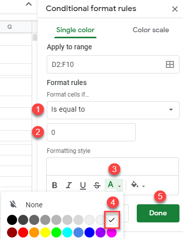
2. In the window on the right side, (1) choose Is equal to under format rule and (2) enter 0. For formatting style, (3) click on the Font color icon, (4) choose the color (white), and (5) click Done.

 

 

You get the same effect again.