Excel or Google Sheets Formula Won’t Calculate
Written by
Reviewed by
This tutorial shows some problems that might prevent a formula from calculating properly in Excel or Google Sheets and how to fix them.
In this Article
Calculation Modes in Excel
By default, when you type a formula into Excel, the result is shown automatically. When the numbers that are affecting the result of this formula change, then the result of the formula is automatically updated. This is because the calculation mode is set to Automatic.
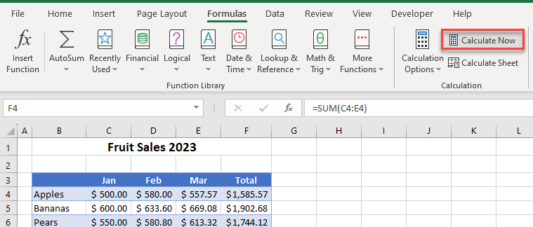
If, however, the calculation mode is set to Manual, then updating the numbers that are used in the formula doesn’t update the formula result unless you manually update the result by pressing the F9 key or by pressing the Calculate Now button on the Ribbon.
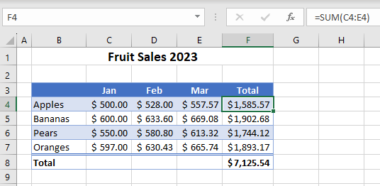
Consider the following data:
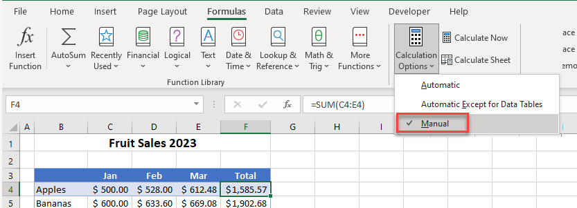
- In the Ribbon, go to Formulas > Calculation > Calculations Options > Manual.
- Then, change the value in one of the cells in the data table that is part of a formula (for example D4).
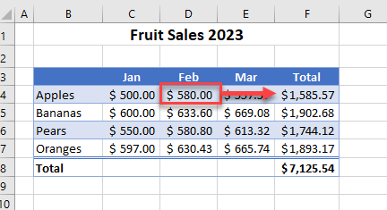
- Note that the formula result in cell F4 does not change. To update the result, press F9. (Or in the Ribbon, go to Formulas > Calculation > Calculate Now.)
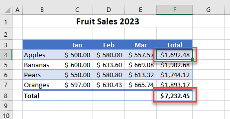
The formula result in cell F4 now reflects the correct result.
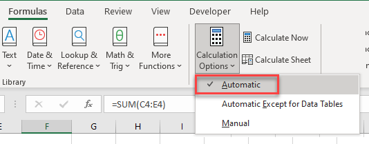
- Click back on the Ribbon and go to Formulas > Calculation > Calculations Options > Automatic to reset to the default calculation setting. (You could also tick Automatic Except for Data Tables.)
- Calculation options in Excel are by default set in the Excel Options menu. In the Ribbon, go to File > Options > Formulas.

Values Formatted as Text
If you import information into Excel, content may come in as text when it is, in fact, numbers. To use these values in a formula, you need to convert them to numbers.
Consider the following data:

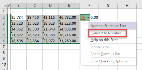
Although there’s a SUM formula in cell F2, intended to add up the range B2:E2, the formula result appears as a zero. This is because the numbers are stored as text. This is indicated by the small green triangle in the top-right corner of each cell where the number is stored as text.
- Highlight the range of cells that are stored as text. This brings up a small yellow triangle to the right of the highlighted cells.
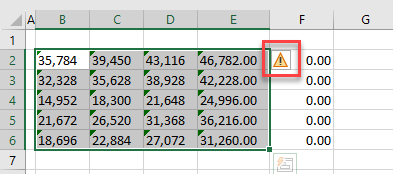
- Click on the yellow triangle to bring up a list of possible solutions to the error and then click Convert to Number.
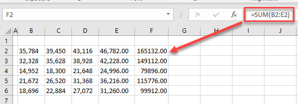
The SUM Function now calculates to show the correct result.
Error Types in Formula Results
If an Excel formula shows an error such #DIV/0!, #REF!, or #NUM!, there is normally a good reason for it. This tutorial explains some of the errors that occur in Excel, shows reasons for each error, and suggests fixes to get the formula to calculate. Read on for common errors that can occur in Excel formulas.
Number Divided by Zero (#DIV/0!)
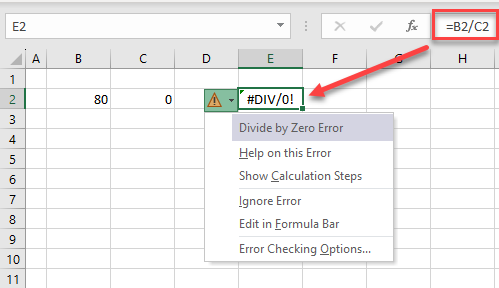
This is caused by a formula where you are dividing a value by zero. If you want to return a zero instead of the #DIV/0! error, use an IFERROR formula.
=IFERROR(B2/C2, 0)
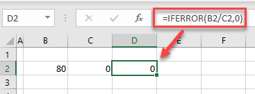
The new formula returns a zero instead of the #DIV/0! error.
No Value Available (#N/A)
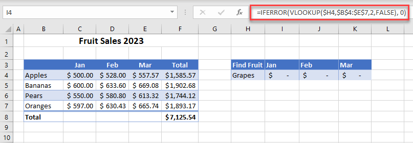
The #N/A error most commonly occurs when using the VLOOKUP, XLOOKUP, HLOOKUP, and/or MATCH Functions.
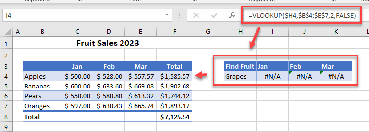
Use an IFERROR formula to replace the #N/A with a zero.
Invalid Numeric Data (#NUM!)
You get a #NUM! error when Excel has a function or formula that contains invalid numeric data or if you have incorrect function arguments.
In the example below, Excel cannot calculate the difference between the two dates because the first date in the formula is after the second date.

To solve this problem, swap the arguments B2 and C2 around in the formula.

You may also encounter the #NUM! error if you are trying to do a calculation that is not possible. For example, if you try to calculate the square root of a negative number, you get this error; it’s not possible to calculate the square root of a negative number!
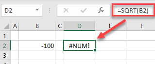
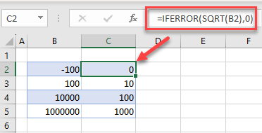
Remove the #NUM! error from the screen by using the SQRT Function in conjunction with the IFERROR Function. Thus, if the number you are trying to get the square root for is less than zero, the formula returns a zero.
Referenced Data Not Found (#NAME?)
Excel lets you create range names. If your formula refers to a range name that does not exist, then you get a #NAME? error.
In the data below, a range name has been created for Apples, Bananas, Pears, and Oranges. The SUM Function has then been used to add up the cells contained in each range name.
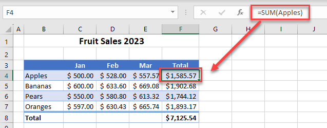
If the range name gets deleted, an error occurs.
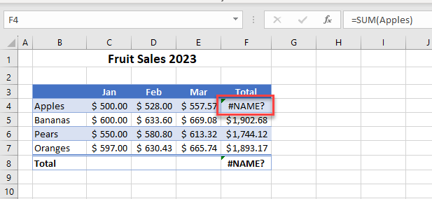
To solve this error, put the range name back in, or edit the formula to use the cell addresses instead of the range name.
Incorrect Syntax (#NULL!)
The #NULL! error occurs when a formula is not correctly written. For example, key signs or symbols are left out of the formula. Below, there’s a missing colon causing the #NULL! error.
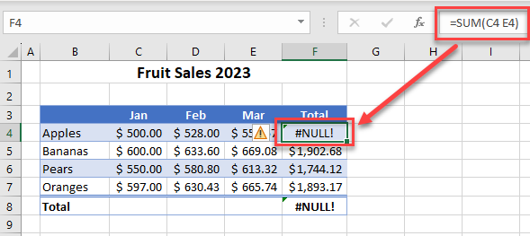
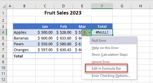
The small yellow triangle indicates an error in the formula and gives you the opportunity to edit the formula in the formula bar.
Dynamic array formulas work by returning multiple results to a range of cells based on a single formula entered in one cell. This is known as “spilling.” A #SPILL! error occurs when a dynamic array formula is being used but the result of the formula is blocked because the spill range isn’t blank.
#SPILL! Error on Sort
The picture below shows an attempt to sort the data in Column B with the SORT Function. However, as there is already data in Column D, you get the #SPILL! error.
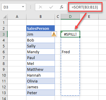
- To fix this error, click the error triangle and choose Select Obstructing Cells.
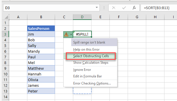
This selects the cell or cells (here, D7) in the way of the spill range.
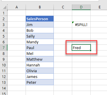
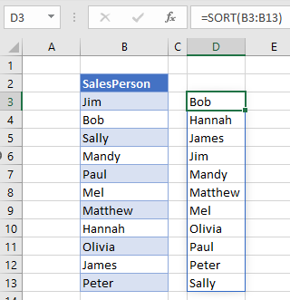
- Clear the data in the obstructing cell or cells so the formula returns the correct result.
#SPILL! Error on Merged Cells
If any of your cells in the spill range are merged, you also get the #SPILL! error.
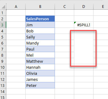
- Once again, click on the green triangle, and choose Select Obstructing Cells to highlight the cells that caused the error.
- Then in the Ribbon, go to Home > Alignment > Merge & Center to unmerge the selected cells.
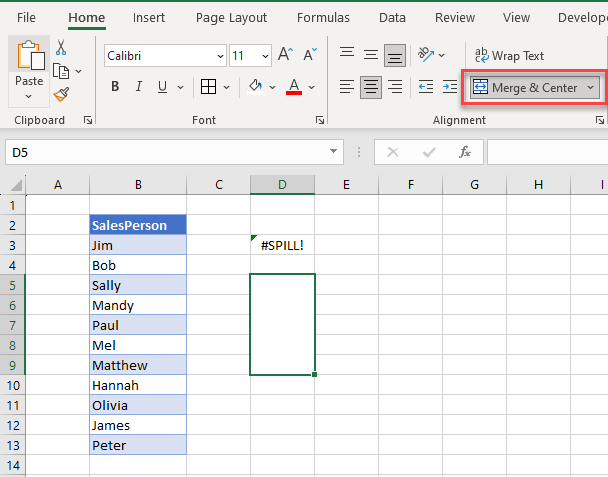
Now the formula returns the correct result.
Tip: Spilled array formulas aren’t supported in Excel-formatted tables, so convert the data to a normal range before attempting to use such a formula.
Invalid Cell Reference (#REF!)
A #REF! error can occur when entire columns of data that a formula refers to are deleted, or when a formula is referring to a range that doesn’t actually exist, such as a broken link.
For example, using the INDEX Function, the function is trying to find a value in Row 5 – which is not included in the array range. This causes a #REF! error.
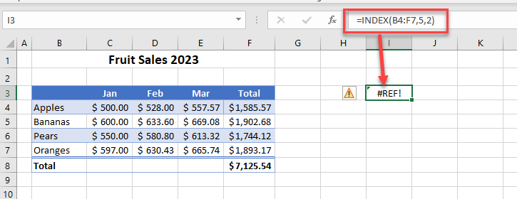
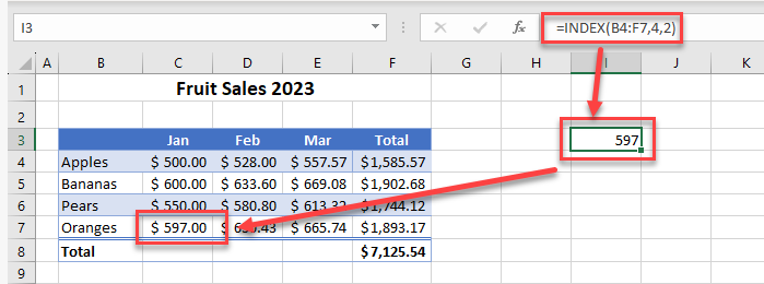
Once the formula is edited (i.e., changing the lookup row argument from 5 to 4), it returns the correct value; there’s no error.
General Error (#VALUE!)
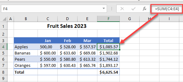
The value error can occur when a formula is trying to calculate numbers, but one of the numbers is actually a text value.
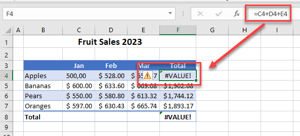
In the example above, the value in cell C4 is text and not a number. The formula is trying to add up C4, D4, and E4. When it picks up that the data in C4 is not a number, you get the #VALUE! error.
To fix this, either change the data in C4 to a value or use the SUM Function instead.
Circular References
If you have a circular reference in your formula, then the formula doesn’t display a result in the cell. The status bar at the bottom of your screen tells you which cell contains a circular reference. Here, it’s cell F4.
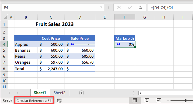
In the picture above, the formula in F4 contains a reference to cell D4 while if you look at the graphic below, the formula in D4 refers to cell F4 thus creating a circular reference. this prevents the formulas in cells D4, F4, and D8 from calculating.

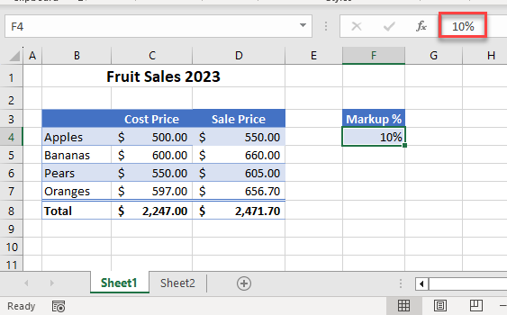
If you remove the formula in cell F4 and replace it with a value, the formulas in cells D4 and D8 now calculate correctly.
Tools in Excel for Solving Errors
Excel has a few error-checking tools available in the Formula Auditing group in the Formulas tab on the Ribbon.

Error Checking
Error Checking in Excel checks your worksheet for any formula errors or circular references.
- If an error shows up in your spreadsheet, you can use the Error Checking command to troubleshoot. In the Ribbon, go to Formulas > Formula Auditing > Error Checking.
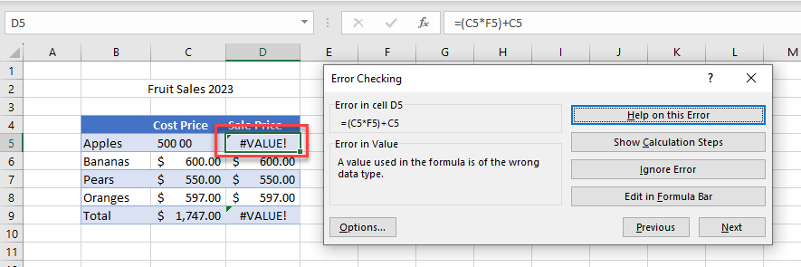
- Click Show Calculation Steps.
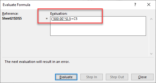
- If you then click Evaluate, the error appears in the Evaluate Formula window.
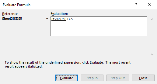
- Click Close and then Edit in Formula Bar to fix the value in the cell (in this instance, there is a space in the value).
Trace Precedents
The Trace Precedents command allows you to trace back to see where the cells are that are contained in your formula. This can help trace errors in workbooks that contain multiple sheets or complicated formulas.
- Click on the cell where the formula is returning an error, and then in the Ribbon, go to Formulas > Formula Auditing > Trace Precedents. This adds arrows to your spreadsheet that point you to the cells that formula references.
- Double-click the blue arrow to move to the corresponding cell. If the cell is in another sheet, double-click the black-dotted line that is shown with a small spreadsheet icon attached.
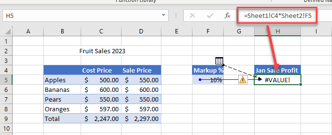
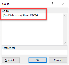
- Click the cell reference in the Go To window, and then click OK to move to that cell.
Google Sheets Formula Won’t Calculate
Most of the error types that occur in Excel also occur in Google Sheets for the same reasons. For example, if you try to divide a value by zero, you get the #DIV/0 in both Google Sheets and Excel. If you are using a lookup function that cannot find a value, the #N/A error occurs, in both applications.
Formula Error (#ERROR)
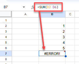
However, there are a few differences. If you make a mistake in a formula in Google Sheets, the cell shows #ERROR.
Invalid Cell Reference (#NUM!)
If your formula is referring to a value that does not exist, you get a #NUM error.

Circular Reference (#REF!)
Should you end up with a circular reference, the error returned on the screen is #REF!
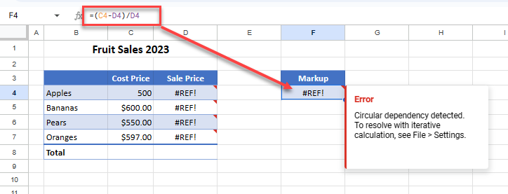
Google Sheets returns an error message as a small red triangle with information on the type of error that occurred. There are no other tracing or error-checking options available in Google Sheets, so these messages are aimed at helping you to determine and solve your errors.

