How to Filter Unique Values in Excel & Google Sheets
Written by
Reviewed by
Last updated on September 5, 2022
This tutorial demonstrates how to filter unique values in Excel and Google Sheets.
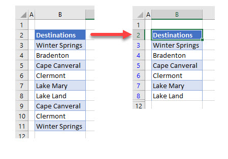
Filter Unique Values With Advanced Filter
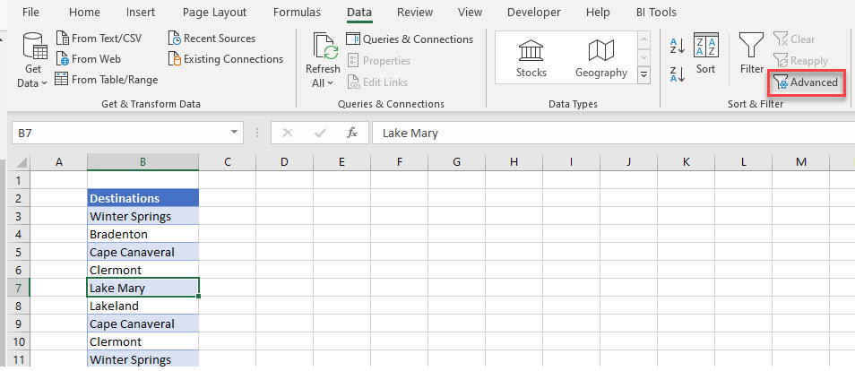
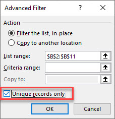
- Click in the list that contains the duplicate values and then, in the Ribbon, select Data > Sort & Filter > Advanced.
- You can either select Filter the list, in place or Copy to another location. For this example, select Filter the list, in place.
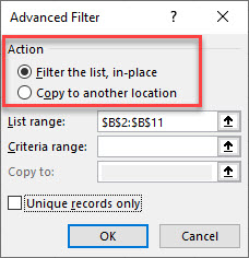
- Then, ensure that Unique records only is ticked and click OK.
The list then shows only unique values, as any duplicate rows are hidden.
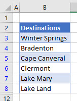
Note: If you select Copy to another location then a list of unique values is placed at the range you have selected the list to be copied to. All the rows in your worksheet are still visible.
COUNTIF and Filter
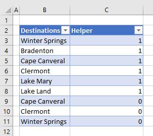
To filter using the COUNTIF Function and standard Filter feature, you need an additional helper column.
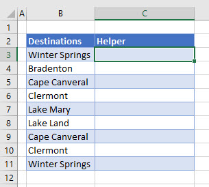
- Click in C3 and type the following formula:
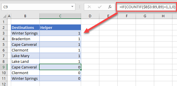
=IF(COUNTIF($B$3:B3,B3)=1,1,0)
- Copy it down to Row 11.
- If the destination appears more than once, a zero appears next to it when it appears for the second or subsequent time.
- In the Ribbon, select Home > Filter.
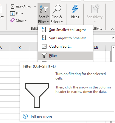
- Drop-down arrows appear in the heading row of your list.
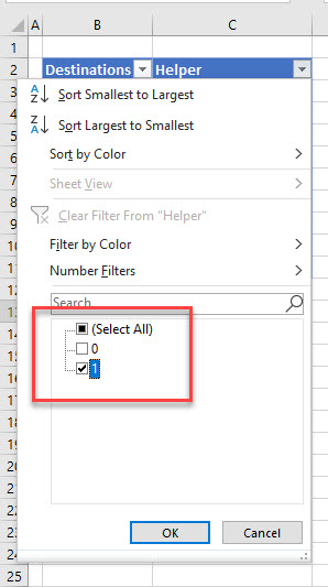
- Click the drop-down arrow in the helper column and select 1 as the value to show.
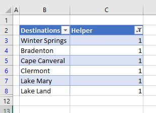
Your list now shows only unique values.
Filter Unique Values in Google Sheets
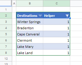
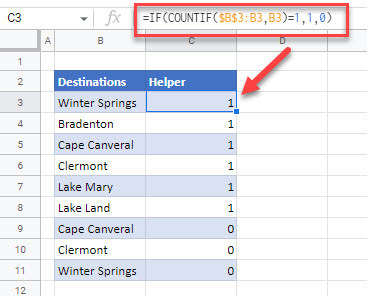
Google Sheets does not have an advanced filter. You can filter duplicate values by using the same formula as you would use in Excel.
- Click in C3 and type the following formula
=IF(COUNTIF($B$3:B3,B3)=1,1,0)- Copy the formula down to Row 11.
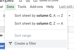
- Select Data > Create Filter from the Menu
- Remove the tick from the 0 so that you filter only on the ones.
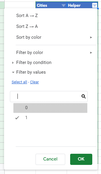
- Click OK to filter the list.
