Dynamic Named Range Based on Cell in Excel & Google Sheets

This tutorial demonstrates how to create and use dynamic named ranges in Excel and Google Sheets.

 

Format Data as a Table

The easiest way to create names for ranges in a spreadsheet is to first format your data as a table.

1. Click in your data, and then in the Ribbon, go to Home > Styles
2. Click Format as Table and choose a style (e.g., Medium > Blue, Table Style Medium 2).

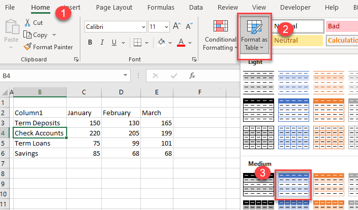
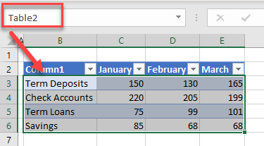
Your data is now formatted as a table, and a Excel adds a new tab (Table Design) to the Ribbon. A new table is automatically given a range name; you can see it in the name box.

Note: The named range does not include the top row if your table has headers.

Dynamic Changes to a Named Table

Click somewhere else in your worksheet and type in the formula:

=Table2

The contents of the table (excluding the header details) show up starting in the cell where you typed the formula.

If you add a row to the table, the table’s named range changes to include that row, and cells linked to the table (i.e., with the formula) update dynamically.

Create Named Ranges From Selection

Excel-Formatted Table

You can add other names for ranges within an Excel-formatted table with just a few clicks.

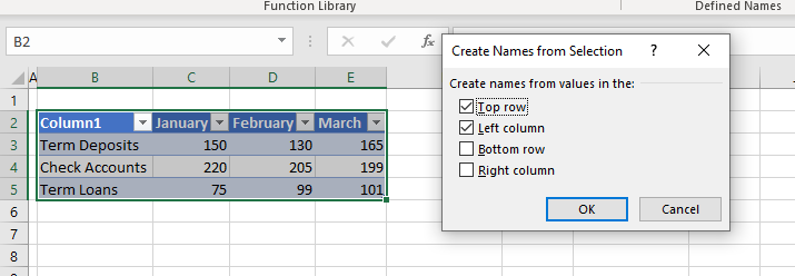
1. Select the entire table, and then in the Ribbon, go to Formulas > Defined Names > Create from Selection.

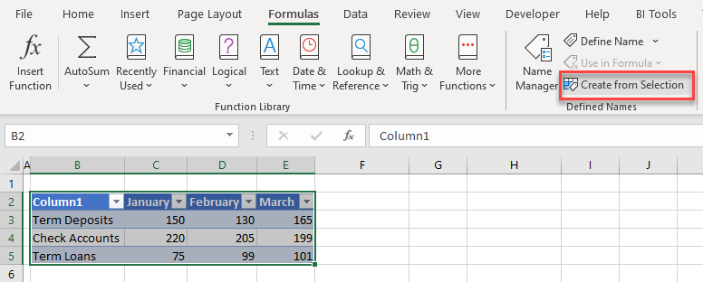
2. Tick the Top row and Left column checkboxes, and click OK.

Dynamic Range Names in an Excel-Formatted Table

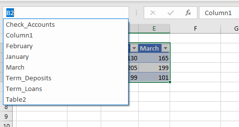
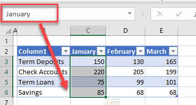
In the name box, you can see all range names that have automatically been created from the selection, including the name of the table.

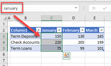
If you choose one of the range names, Excel selects the cells included in that range.

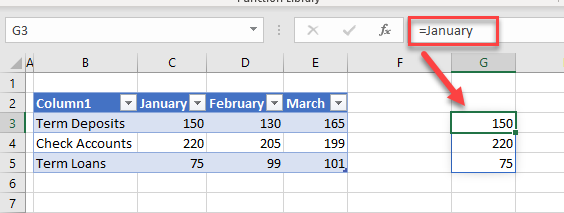
You can use any of the names, just like the table name, in a formula. That formula copies over the entire named range to a new location.

If you add a row to the end of the table, the named range is updated to include the row.

Ranged Table

You can also use Create from Selection to generate range names when your data is not formatted as a table. Select the dataset, and repeat Steps 1 and 2 above.

Tip: Use CTRL + A to quickly select the range.

Dynamic Range Names Without Table Formatting

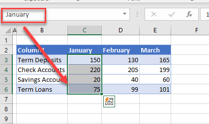
If you add a row to the end of a ranged table, the table’s name does not update to include the row.

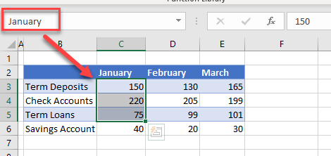
However, if you insert a row into the data, then the named range is updated.

Dynamic Names in Formulas

One of the advantages of using named ranges in formulas is that if the data in the range name changes, the updated data is carried through to wherever the range name has been used.

In the example below, if you change the value for Term Deposits in cell D3, the value in H3 automatically changes.

Dynamic Named Ranges in Google Sheets

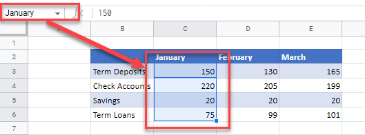
Google Sheets does not have anything like the Excel table feature, but you can still create range names for your data.

1. Select the cells you wish to create a range name for, and then in the Menu, go to Data > Named ranges.

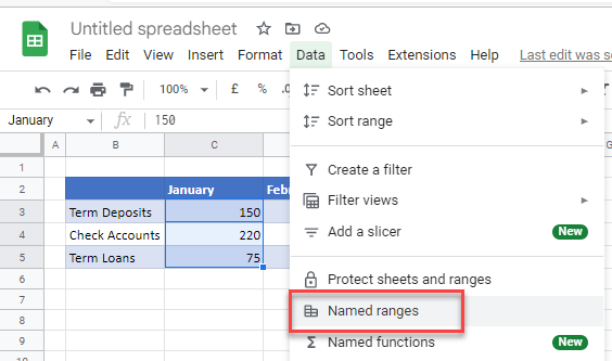
2. Type in the name of the range and then click Done.

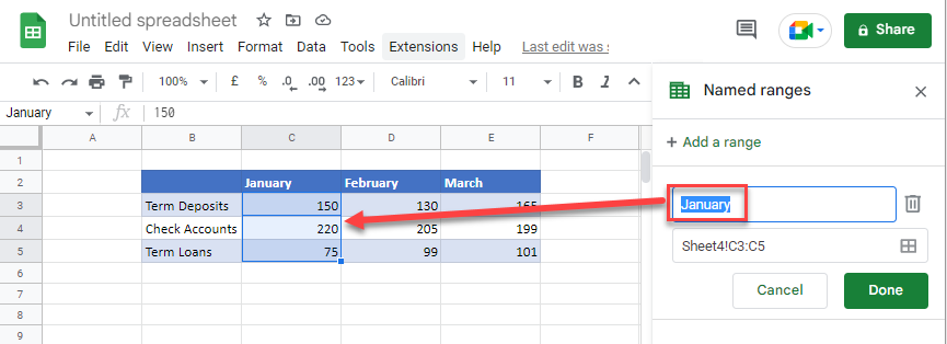
3. You can use this range name in an ARRAYFORMULA. Type this formula into a new cell:

   =ARRAYFORMULA(January)

   The contents of the range name will be inserted into your sheet.

Use Range Names in Google Sheets

If you add a row to the end of the data, the range name does not update, so the added row isn’t automatically included in the named range.

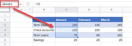
However, if you insert a row, the range name does update.