Drop-Down List with If Statement in Excel

This tutorial demonstrates how to create a drop-down list with an IF statement in Excel and Google Sheets.

Create Custom Drop-Down List (Data Validation)

To create a drop-down list which changes according to what the user chooses, you can use an IF statement within the data validation feature.

1. Select the cell to hold the drop down (here, C2).
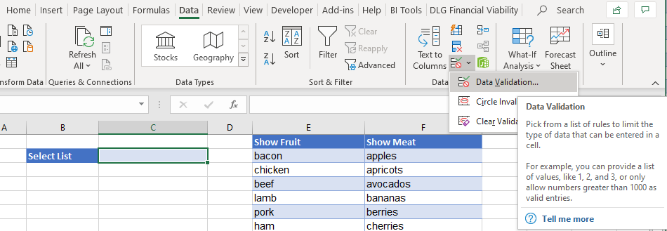
2. In the Ribbon, go to Data > Data Tools > Data Validation.

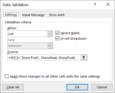
3. Choose List under Allow, and then type in the Source as a formula:

   =IF(C2="Show Fruit", ShowMeat, ShowFruit)

   The formula uses two range names – ShowFruit and ShowMeat. Depending on the option chosen, the corresponding list shows up in the drop-down list. Click OK.

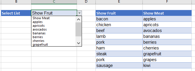
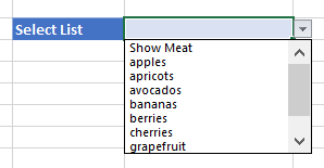
4. Click the arrow to the right of the drop-down list to see the list of available fruit.

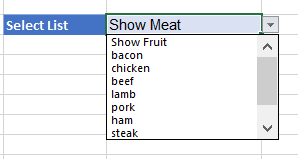
5. Click Show Meat, and then click on the drop-down list again. The list has changed to show the meat list, and the top value has changed to Show Fruit.

Custom Drop-Down List: Nested IF Statement

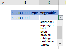
Expand on the formula above by using nested If statements.

1. Select the first drop down’s cell (C2).
2. In the Ribbon, go to Data > Data Tools > Data Validation.
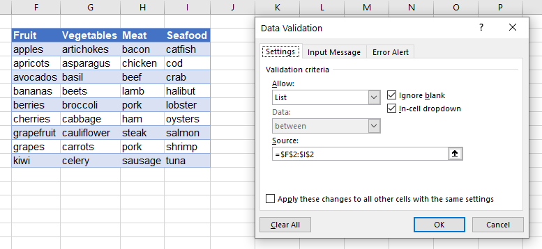
3. Choose List from the Allow drop down, and then set the range (Source) to F2:I2. Click OK.
   Note: In the picture, the range includes dollar signs. This is to lock the range of cells.

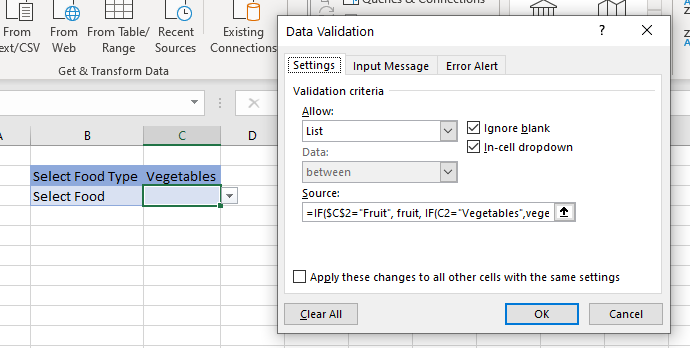
4. Select the cell for the second drop down (C3).
5. In the Ribbon, go to Data > Data Tools > Data Validation.
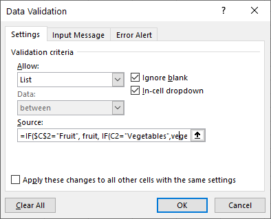
6. Choose List from the Allow drop down, and then type in the formula:

   =IF($C$2="Fruit", fruit, IF(C2="Vegetables",vegetables, IF(C2="Meat", meat, seafood)))

   Once again, the formula uses range names.

7. Choose the food type from the first drop-down list.

8. The list in the second drop-down list changes automatically.