How to Delete Filtered Rows in Excel & Google Sheets

This tutorial demonstrates how to delete filtered rows in Excel and Google Sheets.

 

Delete Filtered Rows

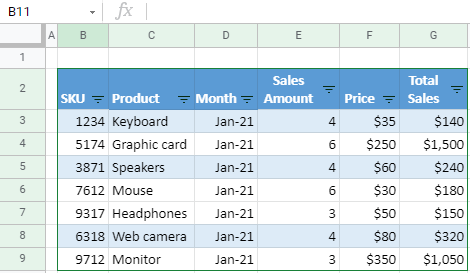
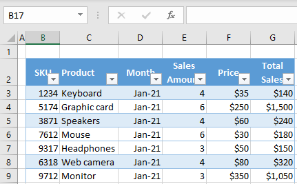
Say you have the set of data shown below and want to delete all rows with the month Feb-21 (Column D).

 

 

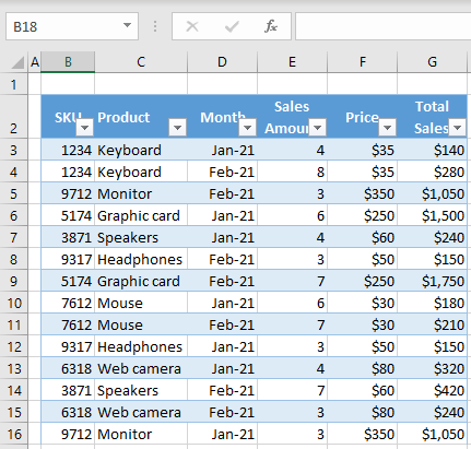
First, Filter the data for Feb-21, and then delete those rows.

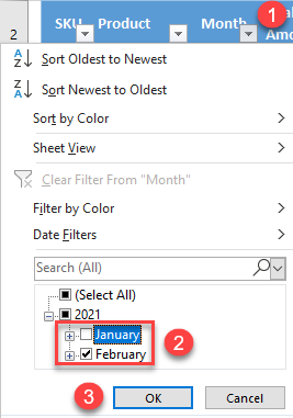
1. Click on the Filter button for Month (cell D2), check only February (uncheck January), and click OK.

 

 

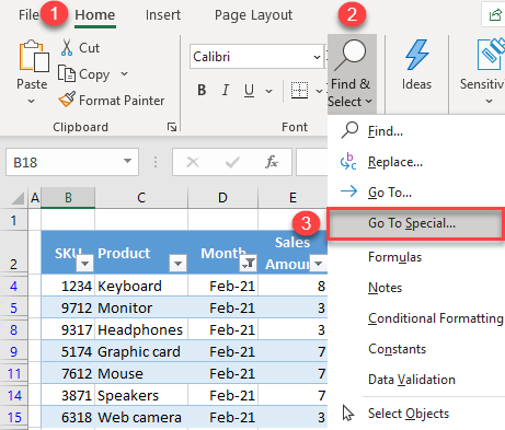
2. Now only the rows with Feb-21 in Column D are visible. To select them, in the Ribbon, go to Home > Find & Select > Go To Special.

 

 

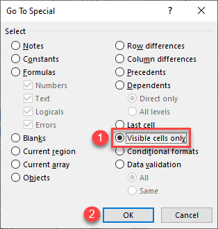
3. In the pop-up window, select Visible cells only and click OK.

 

 

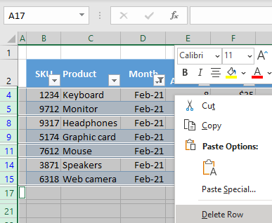
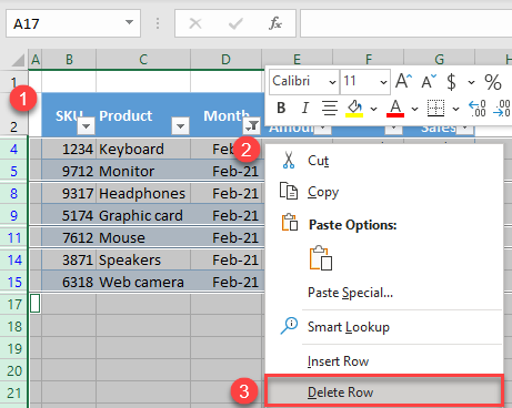
4. Now all rows are selected except for those hidden by the filters. You don’t want to delete Rows 1 and 2, so (1) Hold CTRL and click on those two rows to unselect them.
5. Then (2) right-click anywhere in the selected area and (3) click Delete Row.

 

 

6. Since all visible rows are now deleted, clear all filters to display the hidden rows. Click on the filter icon for Month (cell D2) and choose Clear Filter From “Month”.

 

 

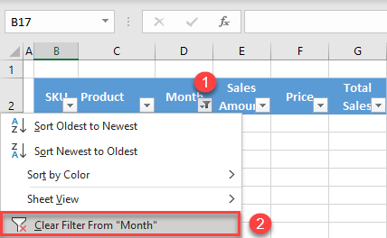
This deleted all rows with the month Feb-21, so only rows with Jan-21 remain in the sheet.

 

 

See also: VBA Delete Entire Row or Column and VBA AutoFilter.

Delete Filtered Rows in Google Sheets

1. Click on the filter button for Month (cell D2), check only February (uncheck January), and click OK.

 

 

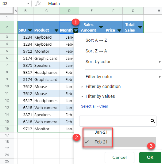
2. Now only rows with Feb-21 in Column D are filtered. Select the filtered rows, right-click anywhere in the selected area, and click Delete selected rows.

 

 

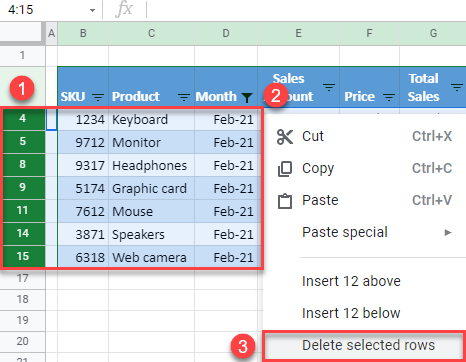
3. As a result of Step 2, rows with Feb-21 in the Month column are deleted. Jan-21 rows remain but are hidden. To unhide them, click on the Filter for Month (D2) and select Jan-21 (or click Select all). Click OK.

 

 

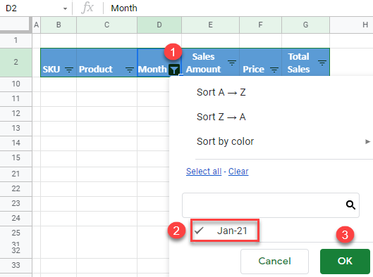
This way, all filters are cleared, and only rows with Jan-21 in Column D are displayed.