How to Use Custom AutoFilter in Excel & Google Sheets

This tutorial demonstrates how to use a custom AutoFilter in Excel and Google Sheets.

 

 

Custom Text AutoFilter

Using a custom text AutoFilter, you can filter a list of data by a specific condition you set (for example, if a cell contains, begins with, or ends with a text or similar). Say you have the following set of data with Product in Column B, and Price in Column C.

 

 

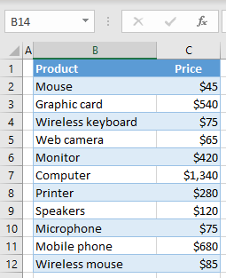
Now you want to filter only rows that contain the word phone in Column B.

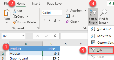
1. First, turn on the filter. Click on any cell in the data range (B1:C12) and in the Ribbon, go to Home > Sort & Filter > Filter.

 

 

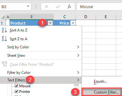
2. Click on the filter button next to Product (cell B1), go to Text Filters, and choose Custom Filter…

 

 

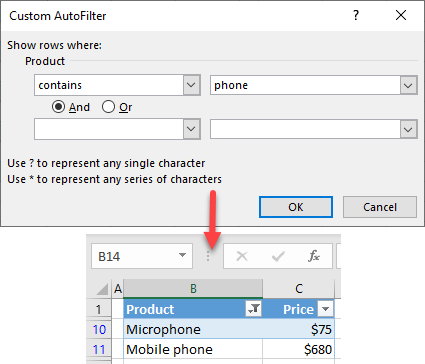
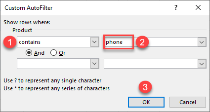
3. In the Custom AutoFilter window, choose contains from the first drop down, type in the text you want to filter (phone), and click OK.

 

 

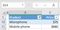
As a result, only Rows 10 and 11 are displayed: Microphone and Mobile phone in Column B, while all other rows are hidden.

 

 

Tip: Learn more about filtering rows with specific text.

Custom Number AutoFilter

Similar to the previous example, you can also create a custom number AutoFilter. For that purpose, you can use the same data range. In this example, let’s filter only products with prices less than $100.

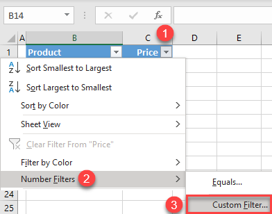
1. Click on the filter button next to Price (cell C1), go to Number Filters, and choose Custom Filter…

 

 

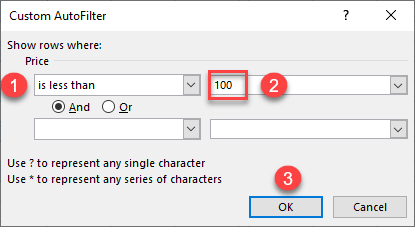
2. In the Custom AutoFilter window, choose is less than from the first drop down, type in the upper limit (100), and click OK.

 

 

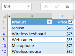
As a result, Rows 2, 4, 5, 10, and 12 are displayed, because these products have a price of less than $100.

 

 

Custom Filters in Google Sheets

 

 

Google Sheets has the standard filter options, and it also lets you create a formula for filtering data. Like Excel, Google Sheets has options when you filter by text:

• text does not contain,
• text starts/ends with,
• text is exactly, and
• custom formula.

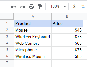
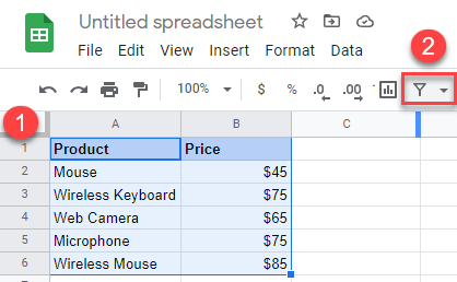
Say you have the following set of data with Product in Column A and Prices in Column B.

 

 

To filter only rows that contain the word Wireless follow these steps:

1. First, turn on the filter. Select the data range (A1:B6) and in the Toolbar, click on the Filter button.

 

 

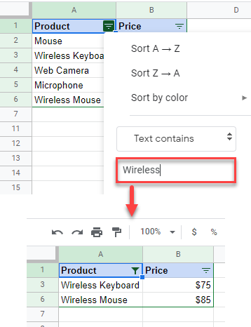
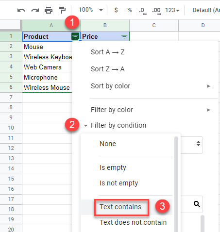
2. Click on the filter button next to Product (cell A1). In the drop down, click Filter by Condition and then Text contains.

 

 

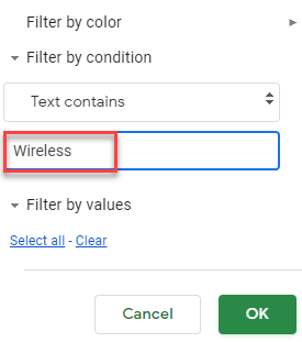
3. In the box enter the text you want to filter (Wireless) and click OK.

 

 

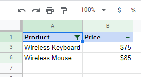
As a result, Rows 3 and 6 are displayed: Wireless Keyboard and Wireless Mouse in Column A, while all other rows are hidden.