Copy Filtered Data (Visible Cells) in Excel & Google Sheets
Written by
Reviewed by
Last updated on September 3, 2023
This tutorial demonstrates how to copy filtered (visible) data in Excel and Google Sheets.

Copy Filtered Data
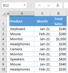
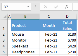
Say you have the following sales dataset and want to filter and copy only rows with Feb-21 in Column C (Month).
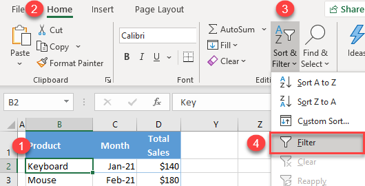
- First, turn on AutoFilter arrows to be able to filter data.
Click anywhere in the data range, and in the Ribbon, go to Home > Sort & Filter > Filter.
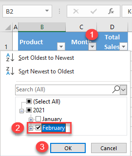
- Now, click the AutoFilter icon for the Column C heading, tick February (under 2021), and click OK.
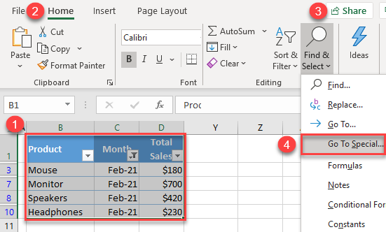
- As a result of previous steps, only rows with the month Feb-2021 are filtered. To copy only visible cells, select the data range you want to copy (B1:D10), and in the Ribbon, go to Home > Find & Select > Go To Special…
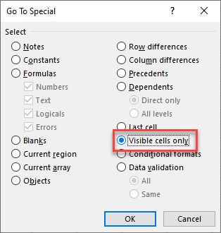
- In the Go To Special dialog box, check Visible cells only and click OK.
-
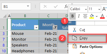
- Now only visible cells (filtered data) are selected. Right-click anywhere in the selected area, and click Copy (or use the keyboard shortcut CTRL + C).
- Right-click the cell where you want to paste the data, and choose Paste (or use the keyboard shortcut CTRL + V).
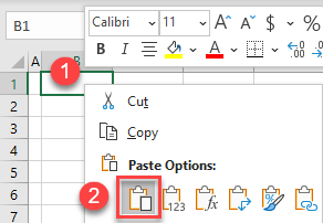
This copies only the filtered data (Feb-21).
Copy Filtered Data in Google Sheets
Say you have the following dataset and want to filter and copy only rows with the word Wireless in Column A (Product).
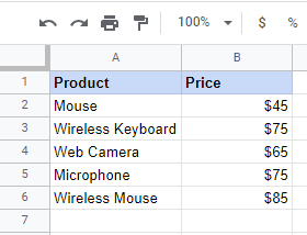
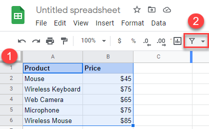
- First, turn on filter arrows. Click anywhere in the data range, and in the Toolbar, click the Filter button.
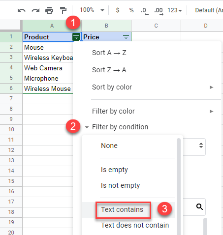
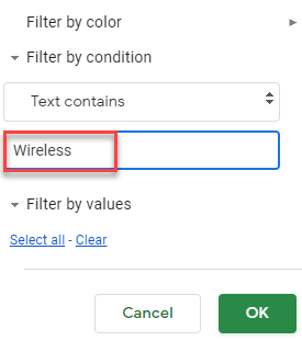
- Now, click on the Filter icon in the Column A heading, click on Filter by condition, and choose Text contains.
- In the box enter the wanted text (in this example Wireless) and press OK.
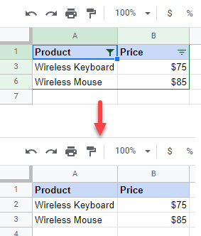
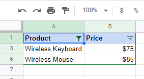
As a result, only rows with the word Wireless are visible.
-
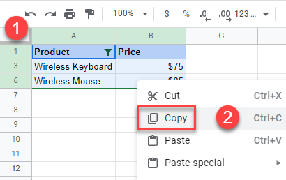
- To copy only visible cells, select the data range you want to copy (A1:B6), right-click it, and choose Copy (or use the CTRL + C shortcut).
- Select the cell where you want to paste the data, then right-click and click Paste.
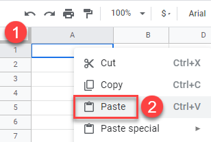
This copies over only filtered data.
