How to Apply the Calculation Style in Excel & Google Sheets

This tutorial demonstrates how to apply the calculation style in Excel and Google Sheets.

Apply Calculation Style

Excel has a variety of predefined styles that you can use to quickly apply formatting to selected cells. Calculation is one of these styles.

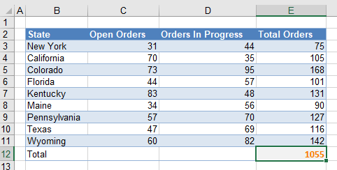
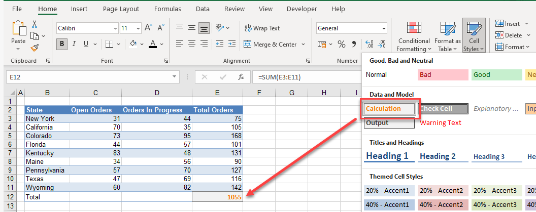
1. To apply the calculation style, first select the cell (here, E12) or cells you want to format as calculation cells.

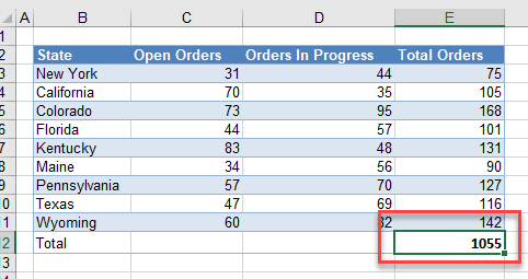
2. In the Ribbon, go to Home > Styles > Calculation to apply the calculation style to cell E12.

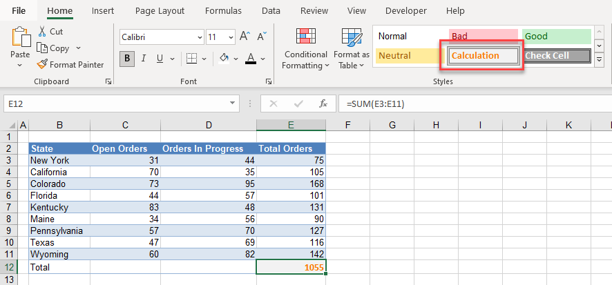
Note: If you don’t see the Calculation style in the Ribbon, go to Home > Styles > Cell Styles.

Then, choose Calculation.

Apply Calculation Style in Google Sheets

Google Sheets does not use styles (though it does use themes), but you can adjust the formatting of each cell to change the background color, font color, and borders. Here’s a workaround for creating and using a “style” in Google Sheets.

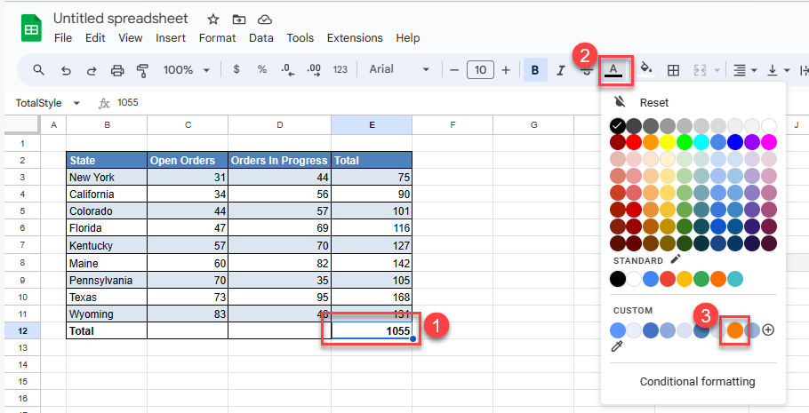
1. First, select the cell you wish to format. In the Toolbar, click the Text Color drop down. Choose a font color for the cell text.

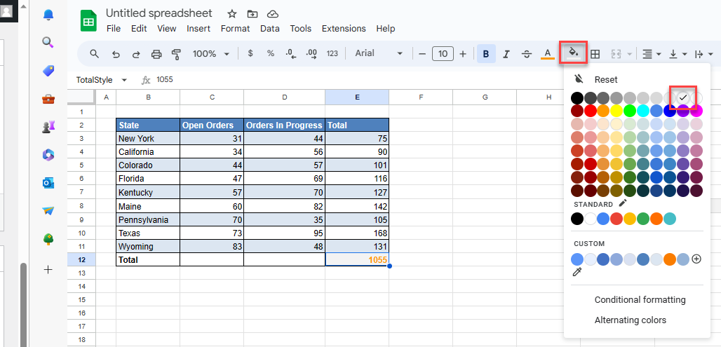
2. Then in the Toolbar, click the Fill color icon and choose a new background color for the cell.

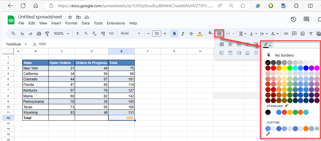
3. If you want to change the color, thickness, or placement of borders, click the Borders drop down in the Toolbar.

• To change the border color, in the Toolbar, go to Borders > Border color, and then choose a color.

• To change the style of the border, in the Toolbar, go to Borders > Border style. Choose a style from different border weights and dashes.

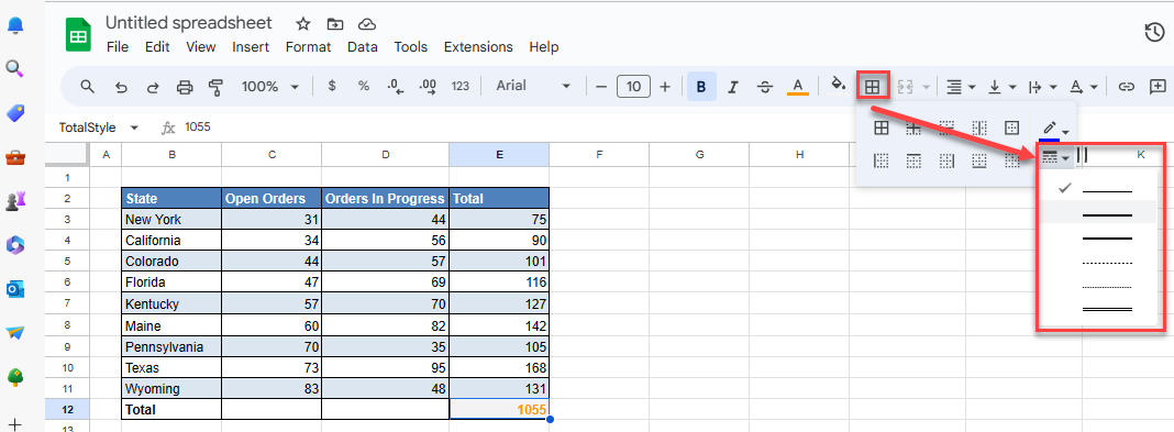
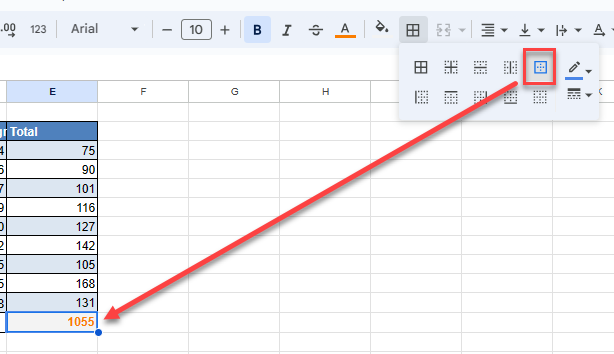
4. Then change the border of the cell by clicking on the type of border.

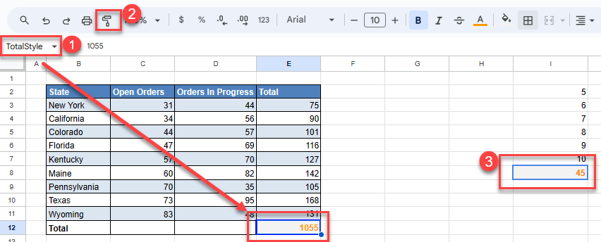
5. For ease of use, name the cell (e.g., TotalStyle) you have applied the format to using the name box.

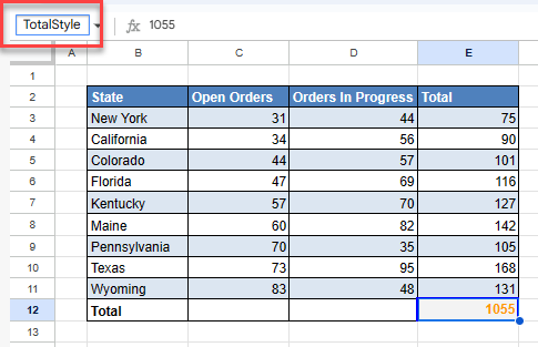
6. Then, if you wish to apply the same formatting to any other cell, first jump to the cell through the name box.
   Click Paint format on the Toolbar, and then click on the cell you want to format.