How to Anchor a Cell in Excel & Google Sheets
Written by
Reviewed by
This tutorial demonstrates how to anchor a cell in Excel and Google Sheets.
A powerful feature of Excel is the ability to copy formulas down and across in a spreadsheet where the cell addresses in that formula automatically change. Sometimes, however, you won’t want cell addresses to change, you may want some to stay static – for example, if you are referring to a specific cell that holds a profit margin or commission rate. When you copy the formula with these cell addresses down or across in the worksheet, you want one (or more) cells referenced regardless of the formula cell’s location. This is known as anchoring the cell or absolute cell addressing.
Anchor Cell References Shortcut
This Excel shortcut cycles through absolute and relative references.
Create Absolute Cell Reference
If you copy a formula down in Excel, the cell references automatically change according to the row.
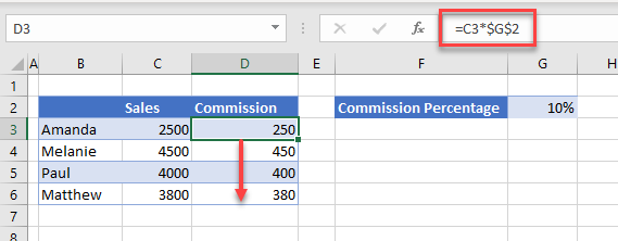
Say you have a worksheet laid out as shown below.

You are working out the sales commission based on a value of 10%, which you are getting from cell G2.
When you copy the formula (=C3*G2) down for the next person’s commission, the formula changes accordingly.

The formula correctly picks up cell C4 (the sales for the salesperson Melanie), but it also moves the cell address down for cell G2. It is no longer picking up the 10% in G2 but is picking up a null value in G3.
To lock the cell (G2) in place, make the cell reference absolute. This means that the cell address does not change when you copy it down or across to the new row or column.
Go back to the original formula, and while still editing it in the formula bar, click on the cell reference (G2) and press F4 on the keyboard to put dollar signs around both the column header and row number in the cell address – so G2 becomes $G$2.
You could also manually put a $ sign before column header ($G) and before the row header ($2) so that it becomes $G$2.

If you copy this new formula (=C3*$G$2) down, the C3 still changes to C4 to pick up the correct sales figures, but G2 stays as is, picking up the cell that contains the commission percentage. This is known as anchoring or locking the cell address; you have created an absolute cell address.

Mixed Absolute References
Occasionally you may wish to only anchor part of the cell address, i.e., either the row or the column, but not both.
Let’s examine the worksheet below.
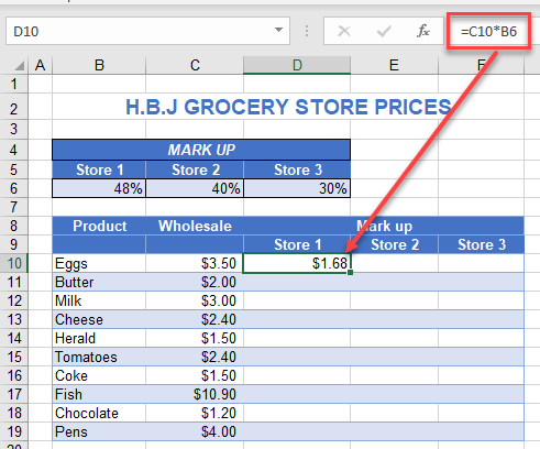
The grocery store has three branches: Store 1, Store 2, and Store 3. Each branch has a different markup percentage for its products. The formula =C10*B6 shows the cost for the first product in C10 (eggs) multiplied by the markup (48%) in cell B6.
If you were to copy this formula down for the rest of the products in Store 1, you would need to anchor the row number for the markup (Row 6) in place. However, to copy the formula across to Columns E and F, you would not need to anchor the column; you want it to pick up the markups in Columns C and D, respectively.
This creates a mixed cell reference; lock the row in place, but not the column.
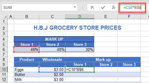
Click back in the formula bar after the cell reference to be anchored (i.e., B6), and put a $ sign before the row number only (e.g., B$6). You can also press F4 twice to toggle from a full absolute reference to a row absolute.
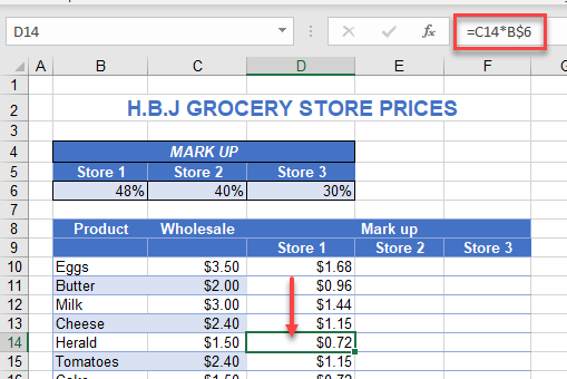
Now, copy this formula down for all products in Store 1.
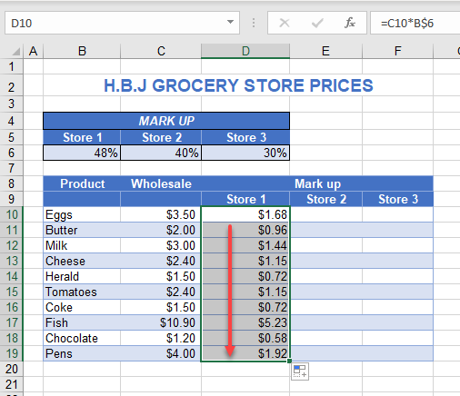
As you copy the formula down, the row for the markup stays the same, as you anchored the row in place.
With the cells still selected, copy the formulas across to Stores 2 and 3.
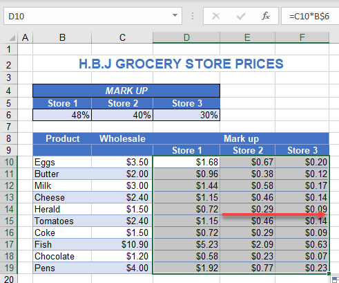
As you copy the formula across, due to the mixed reference, the column changes to pick up the correct store markup – B$6 changes to C$6 and then to D$6, enabling you to enter only one formula for the table.

Anchor Cell in Google Sheets
Anchoring a cell in Google Sheets works exactly the same way as it does in Excel.


