How to Add / Insert a Watermark in Excel

This tutorial demonstrates how to add a watermark in Excel.

Add an Image as Watermark

There are several ways to secure your spreadsheets in digital form, but when it comes to printing them on paper, the best way to mark them for version control is to add a watermark. In Excel, there is no built-in watermark feature, but you can use a workaround and insert it as a picture.

1. In the Ribbon, go to View > Workbook Views > Page Layout.

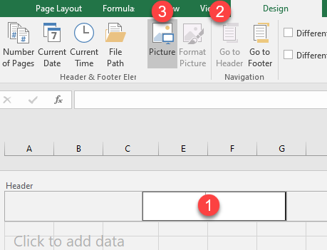
2. Click in one of the three boxes in the header where you want to place your watermark (here, the second box because you want the watermark in the center of the spreadsheet).
   Then, in the Ribbon, go to Design > Picture.

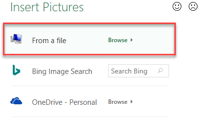
3. This brings up the Insert Pictures window. Choose the location of the watermark image file (here, From a file).

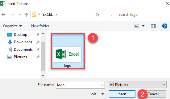
4. Select the image you want and click Insert.

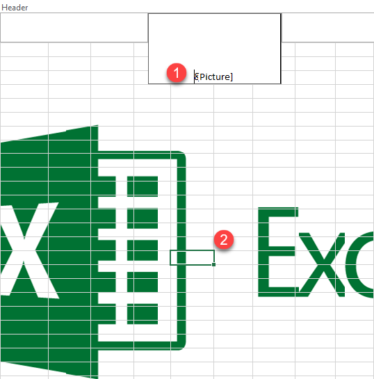
As a result, the picture is added to the header box.

5. Adjust the watermark’s placement by pressing ENTER to lower the position of the picture. To see the watermark on the spreadsheet, just click any cell in the worksheet.

Modify the Image

To make your picture look more like a watermark, make some edits.

1. If the picture is too large, or too small, for the spreadsheet, resize it to fit. In the Ribbon, go to Design > Format Picture.

2. This brings up the Format Picture dialog box. On the Size tab, under Size and rotate, choose measurements that work for your sheet.

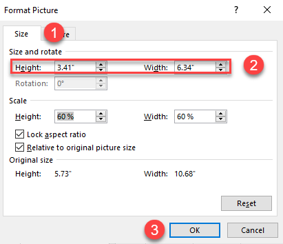
3. In the same Format Picture dialog box, you can adjust the transparency of the picture.
   On the Picture tab, under Image control, change the Color to Washout. Press OK to apply and return to the worksheet.

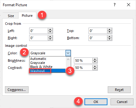
As a result, the picture is now appears as a watermark in Excel.

Add a WordArt Watermark

Another way to add a watermark to your spreadsheet is to insert a WordArt object, but you can only use this option for text-based watermarks.

1. First, in the Ribbon, go to Insert > Text > WordArt.

2. This inserts a text box into your spreadsheet. Type in your text.

3. To format your text and make it look like a watermark, in the Ribbon go to Format > WordArt Styles. Click on the Format Text Effects: Text Box icon (arrow in the bottom-right corner).

4. This brings up the Format Shape task pane on the right side of the workbook. To make the text more transparent, go to Text Options, then click the Text fill and outline icon. Under Color, set the Transparency percent value.

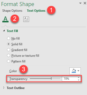
5. To change the dimensions of the text box, in the Ribbon go to Format > Size, and click on the Size and Properties icon (arrow in the bottom right corner).

6. For precise dimensions, in the Format Shape task pane, click on Shape Options, then click on the Size and Properties icon. Under Size, enter the dimensions you need.

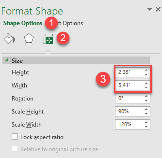
Alternatively, resize the text box directly with the resize handle.

7. To make the text bigger, select it and right-click. In the Font Size box, choose or type in a larger value.

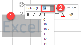
8. To change the text orientation, use the rotation handle.

As a result, you have a watermark added to your spreadsheet with the size, transparency, and orientation you need. Later, if you no longer need the watermark, see how to clear it.

Tip: You can’t add a watermark in Google Sheets, but you can insert a logo to act similarly.