XIRR Function Examples in Excel, VBA, & Google Sheets
Written by
Reviewed by
Download the example workbook
This Excel tutorial demonstrates how to use the Excel XIRR function in Excel to calculate the internal rate of return of a set of cash flows, with formula examples.
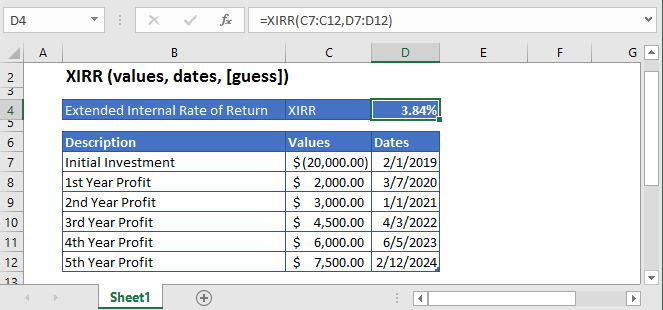
XIRR Function Description:
The XIRR Function Calculates the internal rate of return for a series of cash flows. The cash flows do not need to be periodic.
To use the XIRR Excel Worksheet Function, select a cell and type:
![]()
(Notice how the formula inputs appear)
XIRR Function Syntax and Inputs:
=XIRR(values,dates,guess)values – The values argument consists of an array or a reference to a range of cells representing the series of cash flows. And the values argument must contain at least one negative and one positive value for the calculation.
dates – This argument refers to the array of dates at which the cash flows occur. Its length should be the same as the length of the values array. The first date should be the initial investment’s/loan’s date and subsequent dates of further payments must occur later than the first date.
guess – OPTIONAL: It’s an estimate of what the internal rate of return should be. If this argument is omitted then it assumes the default value of 0.1 or 10%.
What Is Excel XIRR Function?
XIRR stands for Extended Internal Rate of Return. The Excel XIRR function is used to calculate the return on investment in which the series of cash flows occur at specified dates. XIRR Function always returns an annualized IRR value regardless of the intervals of the cash flows.
XIRR Formula
The value of XIRR is calculated as the value of the rate that satisfies the following equation:
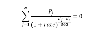
Where:
n = number of time periods
j = period number
rate = discount rate or interest rate
dj = the jth payment or the last payment
d1 = the 0th payment
Pj = the jth payment or the last payment
Calculate Internal Rate of Return of an investment
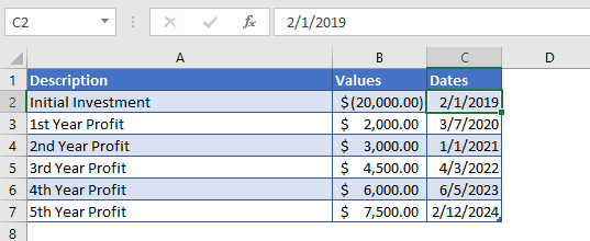
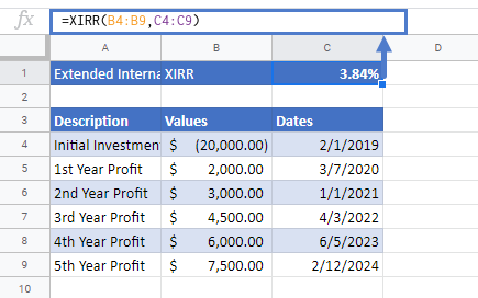
Consider you made an investment of $20,000 in 2019 and expects to receive profits in the next five years. The cash flows and their corresponding dates are mentioned in the above table.
Here the initial investment is entered with a negative sign as this an outgoing payment and profits are represented with positive values. The guess argument was omitted, so the XIRR function operated on the default value of 0.1 or 10%.
The formula used in the calculation of interest rate or internal rate of return is:
=XIRR(B4:B9,C4:C9)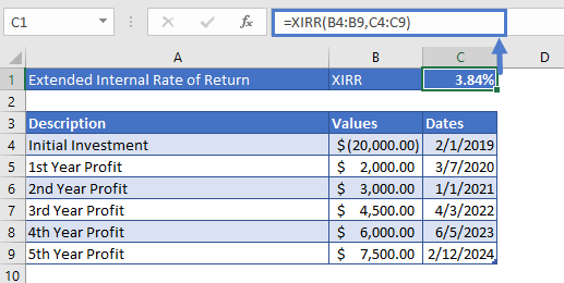
The Internal Rate of Return for this investment is
XIRR = 3.84%
Calculate Internal Rate of Return of a Mutual Fund
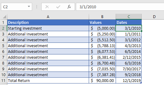
Suppose, you started to invest in a mutual fund with an initial investment of $5,000 in the first year. After seeing good results on your initial investment, you increased your investment by 5% every year, for the next nine years. After nine years, you received a total return of $90,000 on your investments.
In the above table, the first nine values of the Values argument are in negative because it shows payment going out from our account into mutual funds.
The Formula used for calculation is:
=XIRR(B4:B13,C4:C13)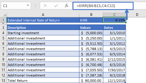
After calculation, the Internal Rate of Return you got on your initial and additional investments is
XIRR = 9.15%
XIRR in Google Sheets
All of the above examples work exactly the same in Google Sheets as in Excel.
Additional Notes
Use the XIRR Function to calculate the Internal Rate of Return of investment.
Cash Flows do not need to be periodic. Instead, you must enter the corresponding dates along with the cash flows.
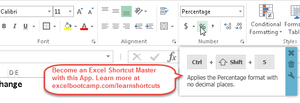
The result of the XIRR Function may appear as a decimal. Change the cell Number Formatting to Percentage to display the function result as a percentage:
XIRR Examples in VBA
You can also use the XIRR function in VBA. Type:
application.worksheetfunction.xirr(values,dates,guess)For the function arguments (values, etc.), you can either enter them directly into the function or define variables to use instead.
Return to the List of all Functions in Excel


