TRIM Function Examples – Excel, VBA, & Google Sheets

This tutorial demonstrates how to use the TRIM Function in Excel, Google Sheets, and VBA to remove all extra spaces from text.

 

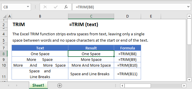
How to use the TRIM Function:

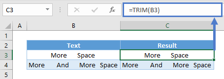
The TRIM function removes all spaces in a text, except for single spaces between words.

=TRIM(B3)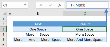

TRIM to Remove Preceding and Trailing Spaces

It can be difficult to spot cells with trailing spaces because text is typically left-aligned: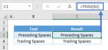

But if you double-click cell B3 or B4, you would see the additional spaces they have by highlighting:

Find Number of Additional Spaces

You may want to find out if the cell has additional spaces instead of doing TRIM right away.

=LEN(B3)-LEN(TRIM(B3))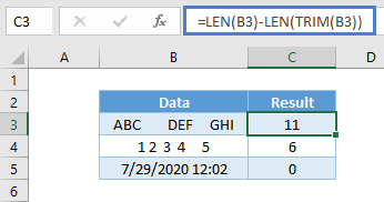

The LEN Function returns the total number of characters in a cell. You can use that to deduct the total length of a trimmed text (removing all additional spaces).

When TRIM Doesn’t Work

You may see obvious additional spaces in the cells, but applying TRIM doesn’t seem to work.

That’s because these are not your typical spaces. All of our characters in the keyboard has a specific ASCII (American Standard Code for Information Interchange) code to it. You could use the CODE Function to find out what is the ASCII code of the character. For eg:

=CODE(B3)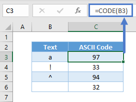

The last one is a regular space in the keyboard and its ASCII code is 32. If you copy one of the “spaces” from where the TRIM doesn’t work and use CODE on it, it show 160:

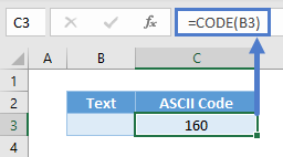
ASCII character 160 is a non-breaking space and usually found in websites and copied to Excel. TRIM only removes character 32 (regular spaces).

To remove the non-breaking spaces and regular ones, you need to combine both the SUBSTITUTE Function and TRIM.

=TRIM(SUBSTITUTE(B3,CHAR(160),""))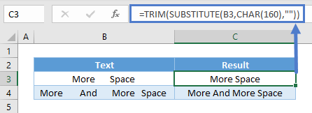

SUBSTITUTE replaces all the non-breaking spaces (ASCII code 160) here with blanks and TRIM removes any additional regular spaces (ASCII code 32) if any.

TRIM with Number/Dates

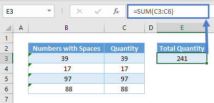
TRIM is a text function. Upon using TRIM, the result is a text. For instance, you won’t be able to sum up these numbers in cell E3 after using TRIM.

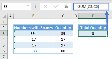
To overcome the issues above, you can use the VALUE Function to convert from text to values.

 

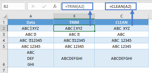
TRIM VS CLEAN

The TRIM Function does not work for non-printable characters, So if you need to remove non-printable characters use the CLEAN Function. Refer to the table below to compare the two functions:

Useful TRIM Function Examples

You can combine TRIM with some of the Excel functions in some useful ways.

Extract Last Word from String

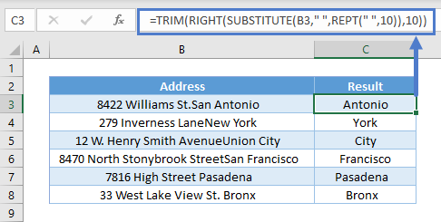
We can combine TRIM, RIGHT, SUBSTITUTE, and REPT to extract the last word from a string (click to see a breakdown of the formula):

=TRIM(RIGHT(SUBSTITUTE(A2," ",REPT(" ",10)),10))

Which would give us the following results:

Find Nth Word in the String

We can combine MID, LEN, SUBSTITUTE, and REPT with TRIM to return the nth word of the string (click to see a breakdown of the formula).

=TRIM(MID(SUBSTITUTE(A$2," ",REPT(" ",LEN(A$2))), (B2-1)*LEN(A$2)+1, LEN(A$2)))

TRIM in Google Sheets

The TRIM Function works exactly the same in Google Sheets as in Excel:

Additional Notes

When working with text, it’s always a good idea to use the TRIM Function to clean the text. Extra spaces can cause unwanted errors when working with functions such as XLOOKUP and MATCH.

You can use the EXACT Function to test if two strings of test are equal. Keep in mind, the EXACT, SUBSTITUTE, and FIND functions are case-sensitive, so it’s also a good idea to use the UPPER, LOWER, or PROPER functions to put all the text in a consistent case.

TRIM Examples in VBA

You can also use the TRIM function in VBA. Type:

application.worksheetfunction.trim(text)

For the function arguments (text, etc.), you can either enter them directly into the function, or define variables to use instead.