SUM Function Examples – Excel, VBA, & Google Sheets

This Tutorial demonstrates how to use the SUM Function in Excel to add numbers.

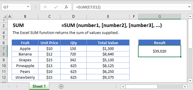
What is the SUM Function?

The SUM Function returns the sum of a range of values. These values can include numbers, cell references, cell ranges, constants, or arrays.

How to Use the SUM Function

You use the Excel SUM Function as follows:

=SUM(C3:C14)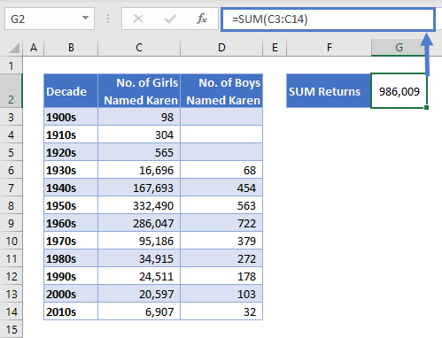

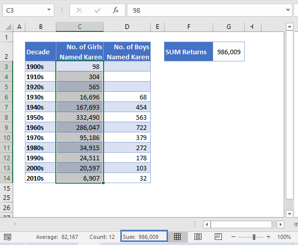
Here we’ve told SUM to add up all of the values in cells C3:C14, which show how many baby girls were named “Karen” in each decade. SUM returns 986,009.

A few points to keep in mind:

• SUM ignores cells containing text
• SUM ignores empty cells
• If a cell in the range contains an error value, SUM will also return an error (use AGGREGATE<<link>> if your cells contain errors)

Using SUM on Multiple Ranges

Now imagine you wanted the sum of all babies named Karen, boys and girls. One way would be to simply extend your range to cover both columns:

=SUM(C3:D14)

But what if the cells weren’t neatly side-by-side, as in the example below?

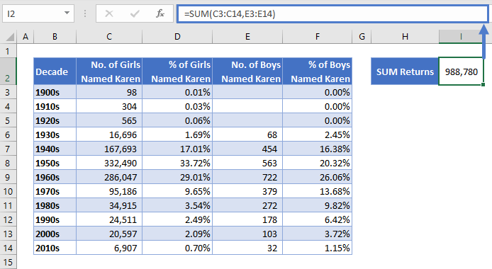
In this case, you can just add a second range to the function, separated by a comma:

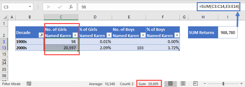
=SUM(C3:C14,E3:E14)

This returns our grand total of 988,780 Karens.

Each of these ranges are called “arguments.” You can define up to 255 arguments in the SUM Function.

SUM Counts Hidden and Filtered Cells

Imagine you wanted to do a quick Karen comparison, one century apart, so you filtered the data to just show the 1900s and 2000s.

See the example below:

As you can see, SUM returns the same result. Even though the other rows are hidden, SUM still includes them, because they are within the range we defined.

If you want to calculate a sum but you don’t want to count hidden or filtered cells, use the AGGREGATE Function instead.

SUM an Entire Column or Row

In the above examples, we specified a set range of cells to sum. But if you’ll need to add data to your spreadsheet in the future, you’ll have to keep updating your SUM functions to make sure they include all the data.

One way around this is to sum the entire column (or row). You do it like this:

=SUM(C:C)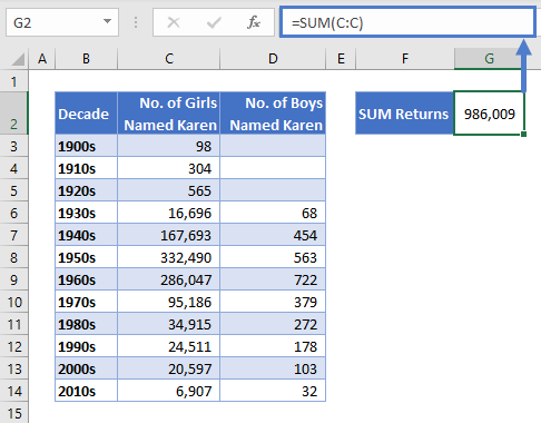

Beware – this will SUM any numerical values in the whole column. Make sure that the column doesn’t contain any data you don’t want to include.

If you want to SUM a row, you’d just specify the row number like this:

=SUM(2:2)

SUM in the Status Bar

Excel very handily shows the sum of any selected numerical range in the status bar, at the bottom of the window below your worksheet tabs.

However, unlike the SUM function, the sum in the status bar does NOT include hidden and filtered cells, as you can see here:

The status bar also shows you the count and the average of the selected range – very useful if you just need to check a statistic quickly.

AutoSum

Very often you’ll want to add a “Total” row to the bottom of your tables. Excel provides an easy way to do that called AutoSum.

Simply select the range you want to sum, click the “Formulas” tab, and then click “AutoSum” in the “Function Library” section.

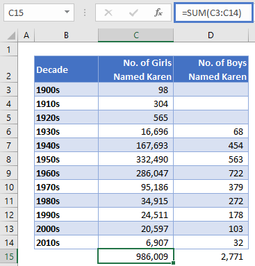
Excel automatically adds a SUM Function at the bottom of each column in your range, showing the sum for that column.

To speed things up even further, you can just use the AutoSum keyboard shortcut: press Alt and the equals = key at the same time.

SUM in Google Sheets

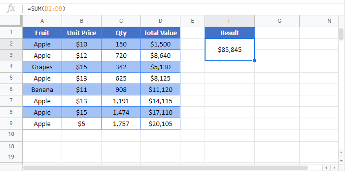
The SUM Function works exactly the same in Google Sheets as in Excel:

SUM Examples in VBA

You can also use the SUM function in VBA. Type:

application.worksheetfunction.sum(number1,number2)