SCAN Function – Excel & Google Sheets
This tutorial will demonstrate how to use the SCAN Function in Excel. (Note: This function is only available in Excel 365.)
Definition
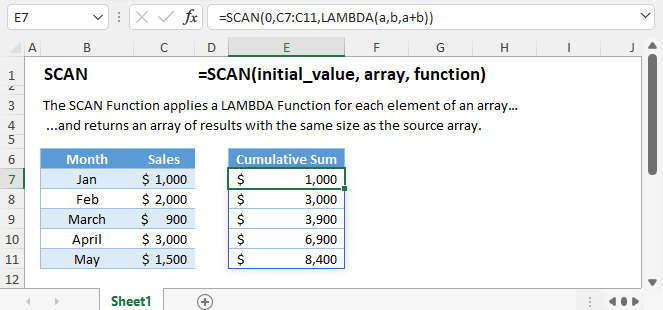
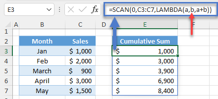
The SCAN Function applies a LAMBDA Function for each element of an array and returns an array of results with the same size as the source array.
=SCAN(0,C3:C7,LAMBDA(a,b,a+b))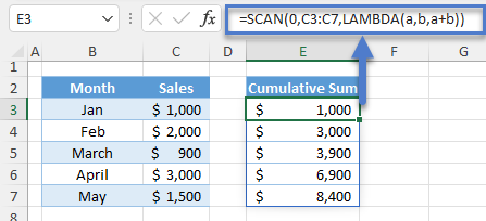
Syntax and Arguments
Here’s the syntax of the SCAN Function:
=SCAN ([initial_value], array, lambda(accumulator, value))Initial_value
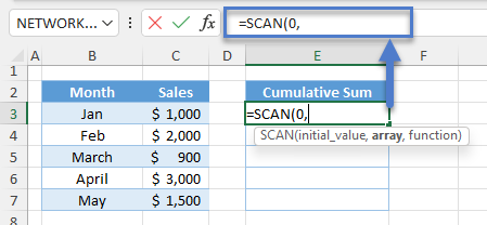
The 1st argument is the initial_value. This argument is the initial value of the accumulator in the LAMBDA Function. It’s an optional input with an empty default value.
Array
The 2nd argument is the array, which is the source array. The SCAN Function will iterate and apply the LAMBDA Function through each element of this given array.
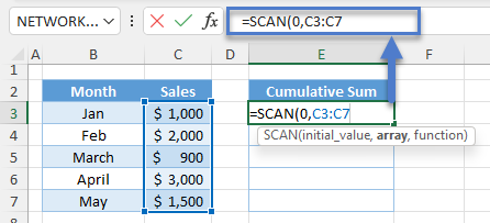
Note: The dimension of the array can be 1D Vertical or Horizontal or 2D.
LAMBDA Function
The LAMBDA Function in the SCAN Function consists of two parameters and one formula:
Accumulator:
In a cumulative summation, the accumulator accumulates its value per iteration, but this is not necessarily true for all scenarios.
The accumulator is technically the output of the previous LAMBDA Function from the previous element.

Note: Its initial value depends on the initial_value argument.
Value
The value is the current array element.
One important property of the value parameter is that it also takes the nature of the array element. If the array is a range, then the value parameter becomes a cell. Therefore, we can use functions that can get cell properties such as the ROW Function.
=SCAN(0,C3:C7,LAMBDA(a,b,ROW(b)))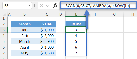
Note: We can use any letters as variables for the accumulator and value.
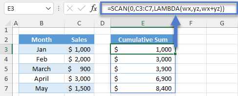
Custom Formula:
We use any formula and nest any function here.
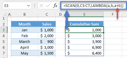
Note: We can omit the accumulator, value or both parameters from the custom formula.
Due to the nature of its LAMBDA Function, most applications of the SCAN Function are related to cumulative calculations. Let’s look at some of the applications.
Cumulative Summation
With the SCAN Function, we can now easily perform an array cumulative summation.
=SCAN(0,C3:C7,LAMBDA(a,b,a+b))
Let’s walk through the formula:
1st Iteration
The accumulator (a) starts with the initial_value.
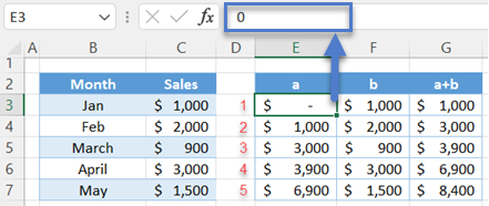
The value (b) starts with the 1st cell in the range.
=C3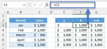
Finally, we calculate the sum of the two.
=E3+F3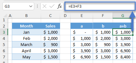
Next Iterations
The accumulator (a) is now equal to the previous output of the LAMBDA Function.
=G3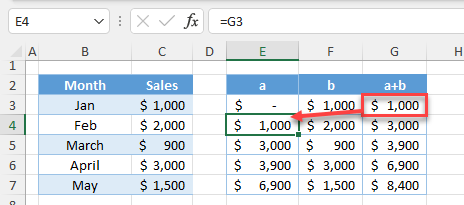
The value parameter (b) is equal to the current element of the array.
=C4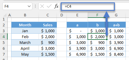
Again, we can calculate the sum of the two.
=E4+F4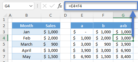
This whole process continues up to the last element of the array.
Cumulative Average
We can also perform a cumulative average using the SCAN Function.
=SCAN(0,C3:C7,LAMBDA(a,b,a+b))/SEQUENCE(COUNTA(C3:C7))
Let’s walk through the formula:
Cumulative Summation
First, we use the SCAN Function to perform an array cumulative summation (see previous section for breakdown).
=SCAN(0,C3:C7,LAMBDA(a,b,a+b))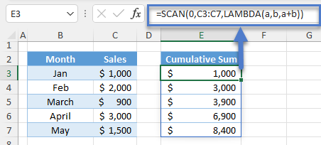
COUNTA Function
Next, we count the total no. of array elements using the COUNTA Function.
=COUNTA(C3:C7)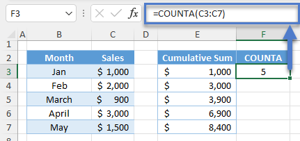
SEQUENCE Function
Then, we use the result of the COUNTA Function to create a vertical list of consecutive numbers using the SEQUENCE Function.
=SEQUENCE(F3)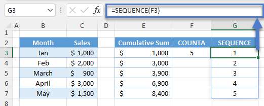
Cumulative Average
Finally, we can calculate the cumulative average by dividing the results of the SEQUENCE Function by the cumulative sum.
=E3/G3
Combining all formulas yields our original formula:
=SCAN(0,C3:C7,LAMBDA(a,b,a+b))/SEQUENCE(COUNTA(C3:C7))
Cumulative Max
We can also calculate the cumulative maximum value using the SCAN Function together with the MAX Function.
=SCAN(0,C3:C7,LAMBDA(a,b,MAX(a,b)))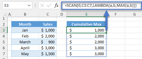
Let’s walk through the formula.
1st Iteration
The accumulator (a) starts with the initial_value.
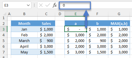
The value parameter (b) starts with the 1st cell in the range.
=C3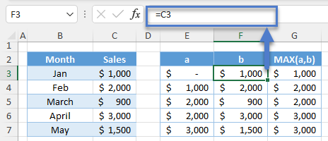
Finally, we calculate the maximum between the two using the MAX Function.
=MAX(E3,F3)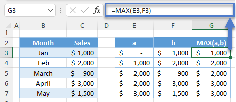
Next Iterations
The accumulator (a) is now equal to the previous output of the LAMBDA Function.
=G3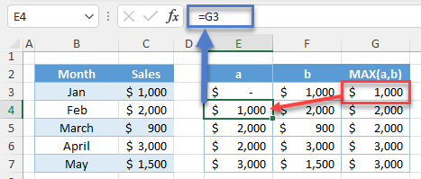
The value parameter (b) is equal to the current element of the array.
=C4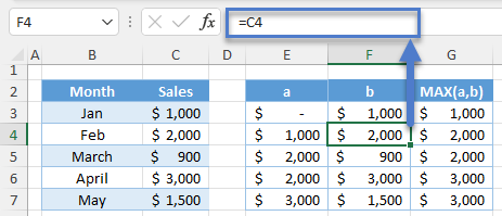
We repeat the MAX Function.
=MAX(E4,F4)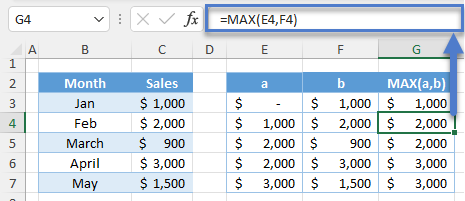
This whole process continues up to the last element of the array.
Cumulative Summation with Reset
There are scenarios where we need to reset the cumulative sum. To do this with the SCAN Function, we use the IF Function to reset the accumulator. Let’s look at the examples.
Year-to-Date Total
One perfect example of a cumulative summation with reset is the year-to-date total. In this case, we need to reset the sum every January of the new year.
=SCAN(0,C3:C16,LAMBDA(a,b,IF(MONTH(OFFSET(b,,-1))=1,b,a+b)))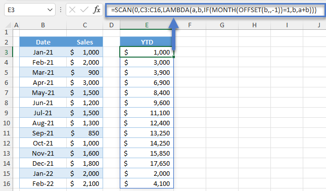
Let’s walk through the formula.
OFFSET Function
Since the array is a range, we can use the OFFSET Function to get the corresponding date from the date column.
=OFFSET(C3,,-1)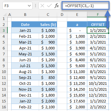
MONTH Function
Next, we use the MONTH Function to get the month number from the date.
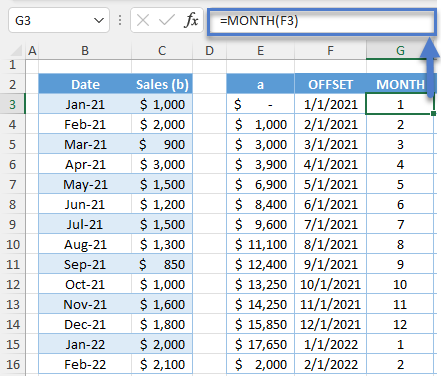
IF Function
Finally, we use the IF Function to check if the month number is 1. If TRUE, we reset the accumulator (a) by returning the current array element (b) instead of calculating the sum (see red highlights). Otherwise, we calculate the sum of a and b.
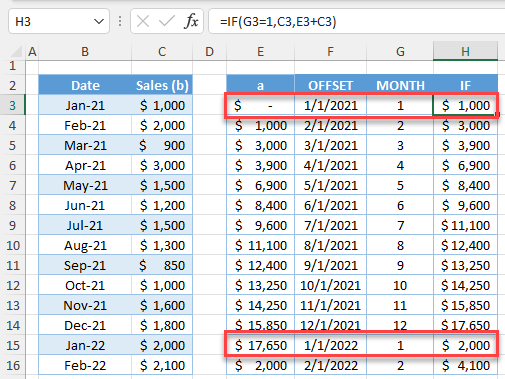
Combining all formulas yields our original formula:
=SCAN(0,C3:C16,LAMBDA(a,b,IF(MONTH(OFFSET(b,,-1))=1,b,a+b)))
Reset every Nth Row
We can also reset the accumulator at every nth row. In the previous case, we must reset the sum every 1st row in a 12-series pattern.
=SCAN(0,C3:C16,LAMBDA(a,b,IF(MOD(ROWS(C3:b)-1,12)=0,b,a+b)))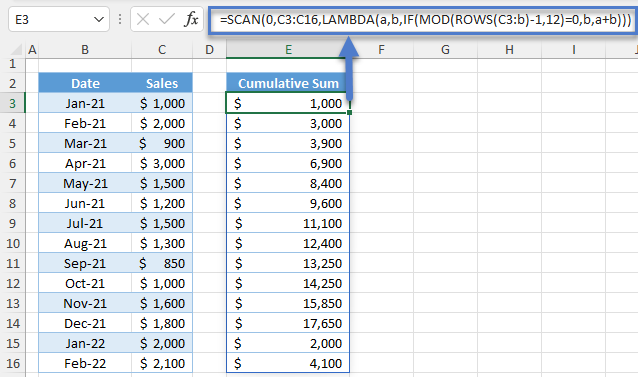
Let’s walk through the formula:
ROWS Function
First, we use the ROWS Function to get the relative row of the value (b) from the first entry (C3) of the array.
=ROWS($C$3:C3)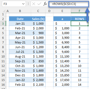
Relative from 0
Next, we deduct 1 from the relative rows to reference the relative rows from 0 instead of 1. The main reason for doing this is for the creation of the 12-series pattern. By starting with 0, we can create a series of consecutive numbers starting with 0 (see next section).
=F3-1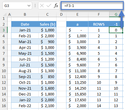
MOD Function
Next, we divide each relative row by the total number of the series pattern, which is 12, and get the remainder using the MOD Function. This creates the 12-series pattern (0 – 11).
=MOD(G3,12)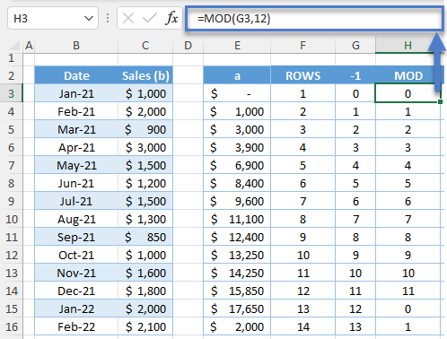
IF Function
Notice that the 1st row of the 12-series pattern is always 0. We now use the IF Function to check for 0 and return the current array element (b) to reset the accumulator (a). Otherwise, we calculate the sum.
=IF(H3=0,C3,E3+C3)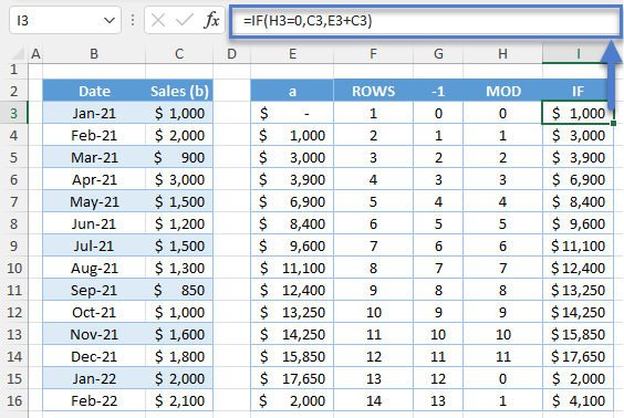
Combining all formulas yields our original formula:
=SCAN(0,C3:C16,LAMBDA(a,b,IF(MOD(ROWS(C3:b)-1,12)=0,b,a+b)))
Cumulative SUM per Row
We can extend the application of the cumulative sum to add another dimension like a cumulative sum per row. In the case below, we take the cumulative sales for each salesperson as the month progresses from January to March.
=SCAN(0,C3:E7,LAMBDA(a,b,IF(COLUMN(b)=3,b,a+b)))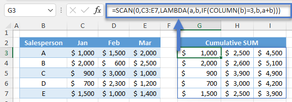
Let’s walk through the formula:
COLUMN Function
First, we use the COLUMN Function to get the column positions of the array elements.
=COLUMN(C3)
IF Function
Next, we use the IF Function to reset the accumulator (a). If the column position is equal to 3 (January Column), then we reset the accumulator to the current array element (b). Otherwise, we calculate the sum.
=IF(J3=3,C3,G3+C3) 
Combining all formulas yields our original formula:
=SCAN(0,C3:E7,LAMBDA(a,b,IF(COLUMN(b)=3,b,a+b)))
SCAN Google Sheets
Currently the SCAN Function is not available in Google Sheets


