RANK Function Examples In Excel, VBA, & Google Sheets

This tutorial demonstrates how to use the RANK Function in Excel to rank a number within a series.

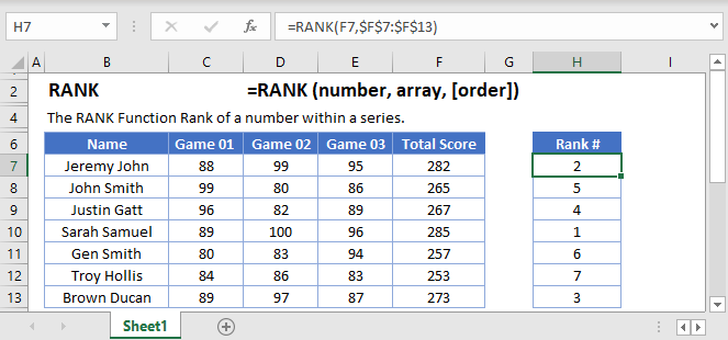
What Is the RANK Function?

The RANK Function calculates the rank of a particular value taken from a data range. That is, how far the value is from the top, or the bottom, when the data is put into order.

RANK Is a “Compatibility” Function

As of Excel 2010, Microsoft replaced RANK with two variations: RANK.EQ and RANK.AVG.

The older RANK Function still works, so any older spreadsheets using it will continue to function. However, you should use one of the newer functions whenever you don’t need to remain compatible with older spreadsheets.

How to Use the RANK Function

Use RANK like this:

=RANK(C8,C4:C13,0)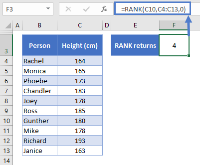

Above is a table of data listing the heights of a group of friends. We want to know where Gunther ranks in the list.

RANK takes three arguments:

• The first is the value you want to rank (we’ve set this to C10, Gunther’s height, but we could also put the value in directly as 180)
• The second is range of data – C4:C13
• The third is the order of the rank
  • If you set this to FALSE, 0, or leave it blank, the highest value will be ranked as #1 (descending order)
  • If you set this to TRUE or any non-zero number, the lowest value will be ranked as #1 (ascending order)

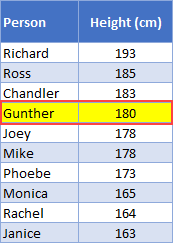
RANK determines that Gunther is the 4^th tallest of the group, and if we put the data in order, we see that this is true:

A few key points about the RANK Function:

• When determining the order, text strings will result in a #VALUE! error
• As you’ve just seen, you don’t need to sort the data for RANK to work correctly

How RANK Handles Ties

In the below table I’ve added a column to the table that returns the rank of each member of the group. I used the following formula:

=RANK(C4,$C$4:$C$13,0)

Note that I’ve locked the data range $C$4:$C$13 by select “C4:C13” in the formula bar, and then pressing F4. This keeps this part of the formula the same so that you can copy it down the table without it changing.

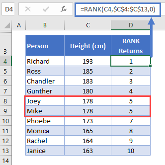
We have a tie! Both Joey and Mike are 178cm tall.

In such cases, RANK assigns both values the highest rank – so both Joey and Mike are ranked 5^th. Because of the tie, there is no 6^th place, so the next tallest friend, Phoebe, is in 7^th place.

How to Use RANK.EQ

RANK.EQ works in the same way as RANK. You use it like this:

=RANK.EQ(C10,C4:C13,0)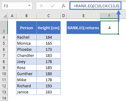

As you can see here, with RANK.EQ you define exactly the same arguments as with RANK, namely, the number you want to rank, the data range, and the order. We’re looking for Gunther’s rank again, and RANK.EQ returns the same result: 4.

RANK.EQ also handles ties in the same way as RANK, as shown below:

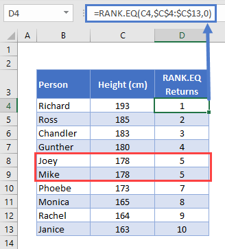
Again, Joey and Mike are tied at 5th place.

How to Use RANK.AVG

RANK.AVG is very similar to RANK.EQ and RANK. It only differs in the way it handles ties. So if you’re just looking for the rank of a single value, all three functions will return the same result:

=RANK.AVG(C6,C4:C13,TRUE)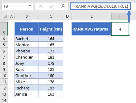

Once again, the same result – 4^th place for Gunther.

Now let’s look at how RANK.AVG differs in terms of ties. So this time I’ve used this function:

=RANK.AVG(C5,$C$4:$C$13,0)

And here are the results:

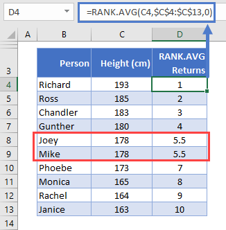
Now we see something different!

RANK.AVG gives Joey and Mike the same rank, but this time they are assigned the average rank that they would have received had their heights not been equal.

So, they would have been ranked 5^th and 6^th, but RANK.AVG has returned the average of 5 and 6: 5.5.

If more than two values are tied, the same logic applies. Let’s pretend Phoebe has a sudden growth spurt, and her height increases to 178cm overnight. Now RANK.AVG returns the following:

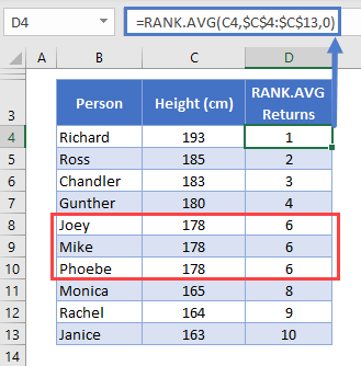
All three friends how rank 6^th: (5 + 6 + 7) / 3 = 6.

RANK IF Formula

Excel doesn’t have a built-in formula that enables you to rank values based on a given criteria, but you can achieve the same result with COUNTIFS.

Say the friends want to create two separate rank orders, one for males and one for females.

Here’s the formula we’d use:

=COUNTIFS($C$4:$C$13,C4,$D$4:$D$13,">"&D4) + 1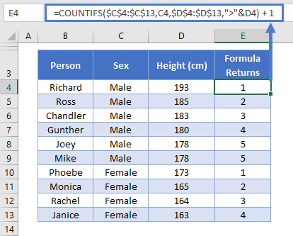

COUNTIFS counts the number of values in a given data range that meet criteria you specify. The formula looks a little intimidating, but it makes more sense if we break it down line-by-line:

=COUNTIFS(
$C$4:$C$13,C4,
$D$4:$D$13,">"&D4
) + 1

So the first criteria we’ve set is that the range in C4:C13 (again, locked with the dollar signs so that we can drag the formula down the table without that range changing) must match the value in C4.

So for this row, we’re looking at Richard, and his value is C4 is “Male”. So we’re only going to count people who also have “Male” in this column.

The second criteria is that D4:D13 must be higher than D4. Effectively, this returns the number of people in the table who’s value in the D column is greater than Richard’s.

Then we add 1 to the result. We need to do this because no one is taller than Richard, so the formula would return 0 otherwise.

Note that this formula handles ties in the same way as RANK.EQ.

Learn more on the main page for the Excel COUNTIF Function.

RANK Function in Google Sheets

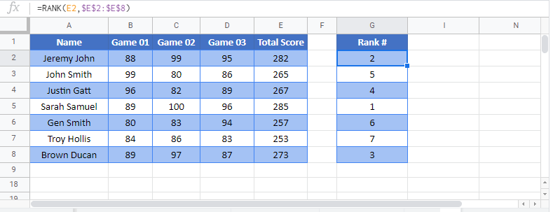
The RANK Function works exactly the same in Google Sheets as in Excel:

RANK Examples in VBA

You can also use the RANK function in VBA. Type:

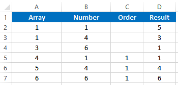
application.worksheetfunction.rank(number,ref,order)

Executing the following VBA statements

Range("D2")=Application.WorksheetFunction.Rank(Range("B2"),Range("A2:A7"))
Range("D3")=Application.WorksheetFunction.Rank(Range("B3"),Range("A2:A7"))
Range("D4")=Application.WorksheetFunction.Rank(Range("B4"),Range("A2:A7"))
Range("D5")=Application.WorksheetFunction.Rank(Range("B5"),Range("A2:A7"),Range("C5"))
Range("D6")=Application.WorksheetFunction.Rank(Range("B6"),Range("A2:A7"),Range("C6"))
Range("D7")=Application.WorksheetFunction.Rank(Range("B7"),Range("A2:A7"),Range("C7"))

will produce the following results