RAND Function Examples – Excel, VBA, & Google Sheets
Written by
Reviewed by
Download the example workbook
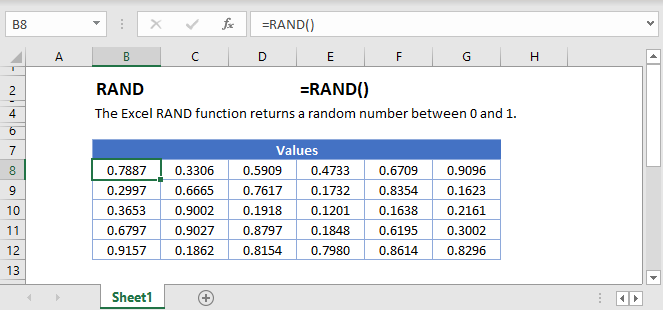
This tutorial demonstrates how to use the RAND Function in Excel to calculate a random number.
How to use the RAND Function in Excel:
The RAND function generates numbers (decimals) greater than 0 and lesser than 1.
=RAND()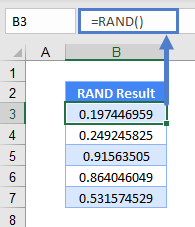
Note: RANDARRAY is a new function in Excel 2019 onwards and replaces the RAND function. But if you don’t have the latest version or need to send the file out for people who don’t have it yet, you still can use the RAND function for backwards compatibility.
Besides generating random numbers greater than 0 and lesser than 1, RANDARRAY allows you to choose how many rows and columns to place the random numbers, choose the minimum and maximum number instead of just 0 and 1, and even choose if you want whole numbers or decimals.
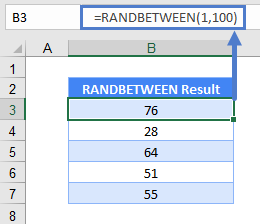
If you have Excel 2007 onwards, you can use RANDBETWEEN as well. Like RANDARRAY, it allows you to choose the minimum and maximum number instead of just 0 and 1. This example below shows random numbers between 1 and 100.
Generate Whole Numbers within a Range
As mentioned, RANDARRAY and RANDBETWEEN do this easily. With RAND, you need to do it like this:
=INT(RAND()*($B$6-$B$3)+$B$3)
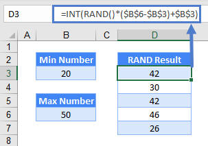
The formula is basically =RAND()*(Maximum Number – Minimum Number) + Minimum Number. And wrap it with an INT to grab the integer.
Generate Random Dates or/and Time
If you know how dates and time are stored in Excel, the logic is going to be the same as above because they are stored as numbers. Just:
=INT(RAND()*($B$6-$B$3)+$B$3)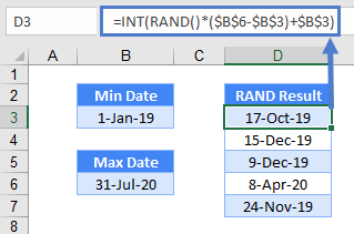
Time is similar, except that it’s decimal instead of a whole number or integer. Hence, remove the INT:
=RAND()*($B$6-$B$3)+$B$3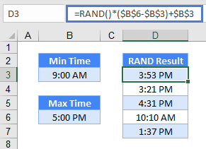
To have them both together, simply add them together:
=INT(RAND()*($B$6-$B$3)+$B$3)+RAND()*($C$6-$C$3)+$C$33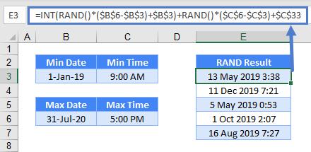
Retrieve a Random Field
If you simply need to randomize decimals, RAND is perfect by itself. Most of the time though, we want to retrieve a random field. To grab a random employee in B3:B7 for instance, you can use a RAND function to assign to each employee, and INDEX and RANK to grab a random employee:
=INDEX(B3:B7,RANK(C3,C3:C7))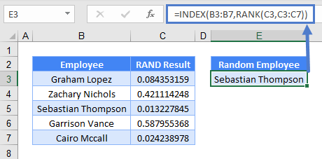
RAND function will randomize numbers in C3:C7. RANK compares the random number in cell C3 among C3:C7 and ranks the number in descending order. 0.0843531593276469 for instance, ranks as number 3 among C3:C7. INDEX grabs the particular row number 3 from B3:B7 and that’s Sebastian Thompson.
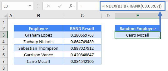
Press the F9 key and the RAND function will recalculate. The value of 0.180669763264754 in cell C3 is now ranked 5 among the numbers in C3:C7 and thus showing the 5th row in B3:B7 and that’s Cairo Mccall.
Do note that while it’s extremely unlikely for RAND function to generate a duplicate number, it’s still theoretically possible.
Retrieve a Random Field without Duplicates
To ensure there are no duplicates, add a COUNTIF to the formula.
=INDEX($B$3:$B$7,RANK(C3,$C$3:$C$7)+COUNTIF($C$3:C3,C3)-1)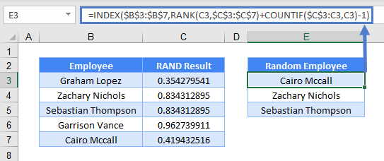
In the above eg, there are two instances of 0.834312895315874. Hence, they both rank the same at 5. With the COUNTIF minus 1 added, the first rank of 0.834312895315874 would be 5 + 1 -1 (5) and the second rank of 0.834312895315874 would be 5 + 2 – 1 (6) and thus pick up different rows.
RAND Function in Google Sheets
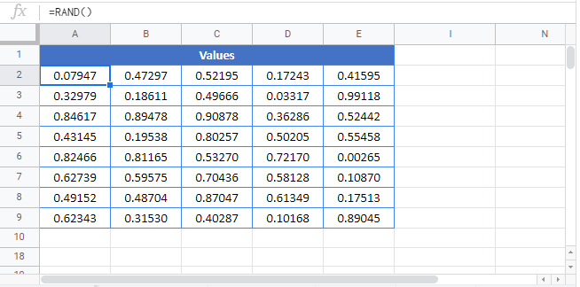
The RAND Function works exactly the same in Google Sheets as in Excel:
