NPER Function – Pmt Period Examples in Excel, VBA & G Sheets
Written by
Reviewed by
Download the example workbook
This tutorial demonstrates how to use the Excel NPER Function in Excel to calculate the number of periods for an investment.
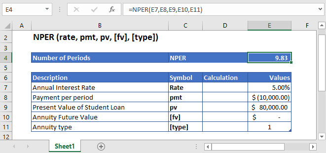
NPER Function Description:
The NPER Function Calculates the total number of payment periods.
To use the NPER Excel Worksheet Function, select a cell and type:
![]()
(Notice how the formula inputs appear)
NPER Function Syntax and Inputs:
=NPER(rate,pmt,pv,[fv],[type])rate – The interest rate for each period.
pmt – It’s the payment per period.
pv – The present value of the investment that future payments are worth now.
fv – OPTIONAL: The Future Value of the investment or loan at the end of the number of payment periods.
type – OPTIONAL: The type argument shows when the payments are made, either at the end of the period by 0 or at the start of the period by 1. Its default value is 0.
What Is NPER?
NPER stands for Number of Periods. It is defined as the total number of periods over which constant payments are made with a constant interest rate.
If the Present Value is given then the NPER is calculated using the following equation:

If the Future Value of the investment is given then NPER is calculated using this equation:
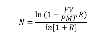
Where:
PV = Present Value
FV = Future Value
R = Rate of Return
PMT = Payment per period
What Is Excel NPER Function?
Excel NPER function helps in calculating the total number of periods required to pay off the loan at a specific interest rate with constant payments.
Calculate the total Number of Periods to pay the student loan
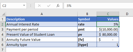
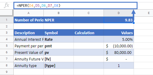
Let’s take a look at an example, where Excel NPER function is used to calculate the total number of payments required to pay off the student loan of $80,000 with an annual interest rate of 5%. The payment of $10,000 is made at the start of each year.
The future value of the investment was not mentioned in the above example, so the [fv] argument is simply omitted or entered with the following value
FV = 0
The payments are being made at the start of the year, so the value of [type] argument is
Type = 1
The formula used for the calculation is:
=NPER(C4,C5,C6,C7,C8)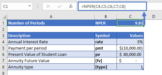
The Excel NPER function returns the following value
NPER = 9.83 years
It would take about 10 years to completely pay off the student loan.
Calculate the Number of periods to get specified return
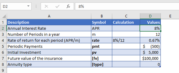
Suppose we invest $5,000 to achieve $100,000 at the end of the investment period. The annual rate of return is 8% and we also make regular contributions of $500, every month. Let’s find out how long it will take us to earn $100,000.
As the payments are made monthly, the annual interest rate is converted into monthly interest by
Monthly Interest Rate – 8% (annual interest rate) / 12 (months per year) = 0.67%
The regular payments being made at the start of the year and it is with a negative sign as it shows outgoing cash
PMT = -$500
The Formula used for the calculation of the number of periods is:
=NPER(D7,D8,D9,D10,D11)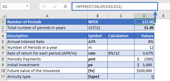
The Excel NPER function returns the following value
NPER = 137.90
As the monthly interest rate was put in the Excel NPER function, the result is also in months. To convert it into years
Yearly number of payments NPER – 137.90 (monthly NPER) / 12 (months in a year) = 11.49 years
It would take about 11 and a half years to get $100,000 investment in return.
NPER in Google Sheets
All of the above examples work exactly the same in Google Sheets as in Excel.
Additional Notes
Use the NPER Function to calculate the number of payment periods of investment.
In the Financial Functions the cash outflows, such as deposits, are represented by negative numbers and the cash inflows, such as dividends, are represented by positive numbers.
NPER Examples in VBA
You can also use the NPER function in VBA. Type:
application.worksheetfunction.nper(rate,pmt,pv,fv,type)For the function arguments (rate, etc.), you can either enter them directly into the function or define variables to use instead.
Return to the List of all Functions in Excel


