MINVERSE Function – Find Matrix Inverse in Excel & Google Sheets
Written by
Reviewed by
This tutorial demonstrates how to use the MINVERSE Function in Excel to return the inverse matrix of a given array.
MINVERSE Function
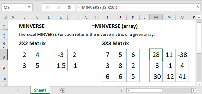
The MINVERSE Function returns the inverse of any array such that it has an equal number of rows and columns.
=MINVERSE(A2:B3)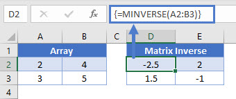
Excel 2019 and Earlier: After entering the formula, instead of pressing ENTER, you must press CTRL + SHIFT + ENTER. This turns the formula into an array. You can identify arrays by the curly brackets surrounding the formula:
{=MINVERSE(A2:B3)}Important: You can not manually type in the curly brackets, this will not work. You must use CTRL + SHIFT + ENTER
Excel 365: In newer versions, you no longer need to use CTRL + SHIFT + ENTER. You can simply press ENTER.
MINVERSE Function – Non-Square Matrix
The MINVERSE Function will return an error if the array is not a square matrix.
= MINVERSE(A2:B4)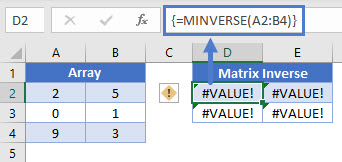
MINVERSE Function – Text or Empty Cell
The MINVERSE Function will also return an error if any member of the array is either empty or contains some text.
=MINVERSE(A2:B3)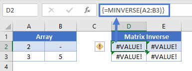
MINVERSE in Google Sheets
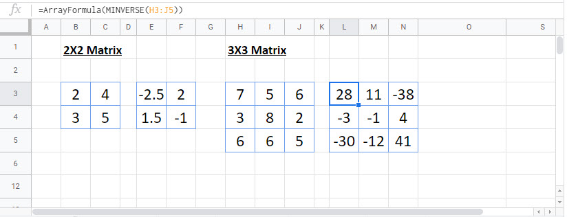
The MINVERSE Function works exactly the same in Google Sheets as in Excel:
