LINEST Function Examples in Excel, VBA, & Google Sheets

This tutorial demonstrates how to use the LINEST Function in Excel to calculate statistics about a trendline.

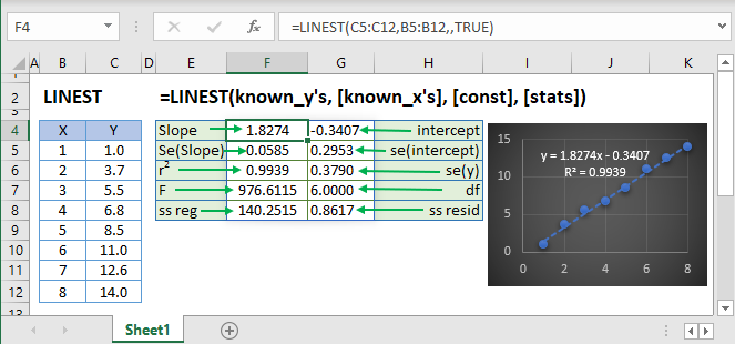
What is the LINEST Function?

The LINEST function in Excel is a function used to generate regression statistics for a linear regression model. LINEST is an array formula and can be used alone, or with other functions to calculate specific statistics about the model.

Linear regression is a method in statistics used for predicting data following a straight line using known data. Regression is used to predict values such as sales growth, inventory requirements or simple market trends.

LINEST is like FORECAST in that it achieves a similar outcome, but with far more information about your regression model as well as the option to fit more than one independent variable.

Suppose I have a table of data with x and y values where x is the independent variable and y is the dependent variable:

I want to know what the regression equation of the above data is. Using LINEST:

=LINEST(B3:B7,C3:C7,TRUE,FALSE)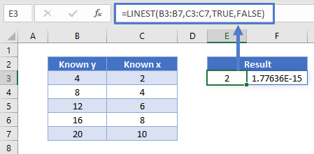

The y-intercept value here is equivalent to 0, in scientific notation.

The equation of the line is y= 2x + 0 . Note that LINEST returns both the slope and intercept of the line. To return both values, the formula must be entered as an array formula. More on array formulas later.

How to use LINEST

The LINEST function takes four arguments:

=LINEST(known_y’s, known_x’s, const, stats)

Where,

Argument	Description
known_y’s and known_x’s	Is the x and y data in your data table
const	TRUE/FALSE option for whether the y-intercept should be forced to 0 or calculated normally
stats	TRUE/FALSE option whether additional regression statistics should be returned

 

Using our first example, the function is written as:

=LINEST(B3:B7,C3:C7,TRUE,FALSE)

When the stats option is set to TRUE, the organization of the regression statistics are as follows:

You may be wondering what each variable means.

Statistic	Description
mn	Slope coefficients for x variables
b	y-intercept
sen	Standard error for each slope coefficient
seb	Standard error for the y-intercept
r2	Coefficient of determination
sey	Standard error for the y estimate
F	The F statistic (to determine if the variables’ relationship occurs by chance)
df	Degrees of freedom
ssreg	Regression sum of squares
ssresid	Residual sum of squares

The main statistics to understand are the slope coefficients, y-intercept and the coefficient of determination or the r² value of the model.

Using the above example and selecting TRUE for the stats parameter:

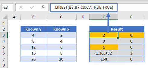
The highlighted cells show the slope = 2, intercept = 0 and r² = 1.

The r² value is an indicator of the strength of the correlation of the model. It can be thought of as an indicator of fit. A low r² value would mean a poor correlation between your dependent and independent variables, and the opposite is true for high r² values, with r² = 1 being a perfect fit.

In releases following January 2020 of Excel in Microsoft 365 (previously Office 365), dynamic arrays have changed the way array formulas are evaluated. It is no longer required to use CTRL + SHIFT + ENTER or highlight the area of cells the array will take up. Simply enter the formula and click enter and the resultant cells will “spill out” into the array.

For the remainder of this article we will reference using LINEST with respect to dynamic arrays in Microsoft 365 Excel.

Forecasting with LINEST (Simple Regression)

Combining the LINEST and SUM functions can be used to predict the value of a dependent variable y, given known x and y data. Below is an example showing what the y value will be when x=14.

=SUM(LINEST(C3:C7,B3:B7)*{14,1})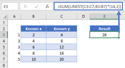

The model comes in the form y =mx + b . This is the same as y = a+ bx, just a different way to represent the equation. A tip to keep in mind for linear equations is the variable next to x is always the slope, and the variable following a plus or minus sign is always the intercept, regardless of the letters used in the equation.

Using the formula: =SUM(LINEST(C3:C7,B3:B7)*{14,1})returns the result of 28. Since this is a single result, it is not necessary to enter as an array.

The tail end of the above formula *{14,1} specifies the independent variable to be used for predicting the dependent variable, in this case, 14.

We can check this by entering  x= 14 in the equation of the line, y =2x + 0.

Forecasting with LINEST (Multiple Linear Regression)

The following data table comes from the Microsoft Support website LINEST page.

In some cases, there is more than one independent variable which should be considered when creating a linear regression model. This is called multiple linear regression (i.e. multiple independent variables). If I want to estimate the cost of an office building, things like floor space, number of building entrances, age of building and the number of offices would all be part of the equation. Let’s see an example.

Typing the LINEST formula into cell G29 and executing it, we get:

=LINEST(E3:E13,A3:D13,TRUE,TRUE)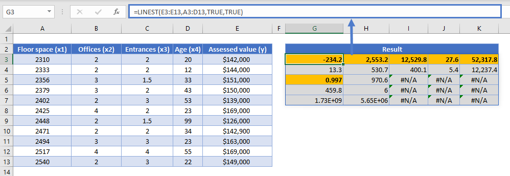

The model comes in the form:

Remember that the LINEST result array is in reverse order from the equation. In the above example, 52,317.8 is our intercept, b, and 27.6 is our m₁ or the slope value for the Floor space variable, x₁.

Using the LINEST function with the data provided, our regression model is:

With an r² value of 0.997, which indicates a strong or highly correlated model. Using the model, you can now predict what the assessed value of an office building will be based on any combination of the above independent variables.

LINEST Tips

1. If you are on a non-Microsoft 365 release, you will have to use the legacy CTRL + SHIFT + ENTER (CSE) method of evaluating array formulas.
2. If using the legacy method, the number of columns to highlight when entering a LINEST array function is always the number of x variables in your data plus 1. The number of rows to select for the array is 5.
3. If you will be sharing your dynamic array enabled version of Excel with someone who is using a non-Microsoft 365 release, use the legacy CSE method to avoid compatibility issues.

Interested in More Forecasting?

See our other articles on Forecasting with Exponential Smoothing, TREND, GROWTH and LOGEST functions.

LINEST function in Google Sheets

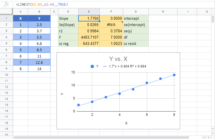
The LINEST function works exactly the same in Google Sheets as in Excel.

LINEST Examples in VBA

You can also use the LINEST function in VBA. Type:

application.worksheetfunction.linest(known_ys,known_xs,const,stats)

Executing the following VBA statement

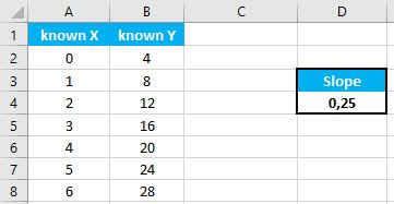
Range("D2") = Application.WorksheetFunction.LinEst(Range("A2:A8"), Range("B2:B8"))

will produce the following results: