LEFT Function Examples – Excel, VBA, & Google Sheets

This tutorial demonstrates how to use the LEFT Function in Excel and Google Sheets to return the first n number of characters in a cell.

How to use the LEFT Function in Excel:

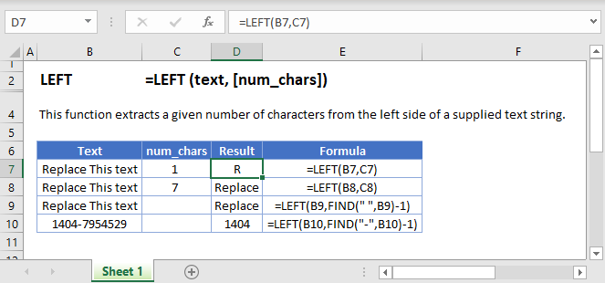
The LEFT function extracts a specific number of characters you specify from the left (start of the string).

=LEFT(B3,C3)

The above extracts 7 characters from the left or the start of the string.

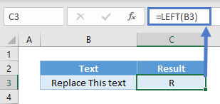
The second argument is optional and the default value of it is 1. Hence, it extracts 1 character from the left and gives you “R” if you omit it.

LEFT with FIND/SEARCH

In many scenarios, the number of characters we want to extract from the left varies just like first names. In this case here, we can use FIND to check which character position the space starts and minus one to exclude the space itself.

=LEFT(B3,FIND(" ",B3)-1)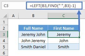

You can also use SEARCH. The difference between FIND and SEARCH is that the former is case-sensitive. Finding a symbol such as space wouldn’t matter.

=LEFT(B3,SEARCH(" ",B3)-1)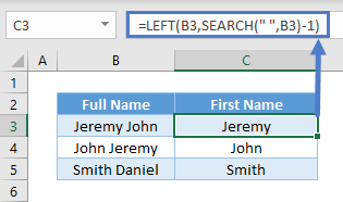

LEFT with LEN

There could be instances where you know how many characters you don’t want, but not how many you want. In the example below, there are always 4 numbers at the end. But the number of alphabets differ.

=LEFT(B3,LEN(B3)-4)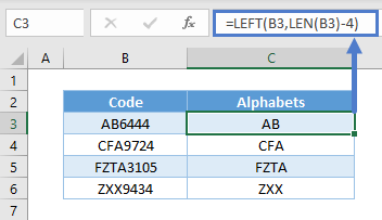

LEN helps us obtain the total number of characters in the cell. And since we know we don’t want the 4 numbers at the end, simply use total length minus 4 characters to obtain the number of alphabet characters.

LEFT with Numbers or Dates

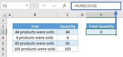
LEFT is a text function. Upon using LEFT, the result is text. For instance, you won’t be able to sum up these numbers in cell E3 after using LEFT.

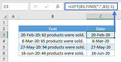
The same thing happens for dates as they are recognized as serial numbers and not text. You may not need to sum dates, but it doesn’t work well in filters and PivotTables.

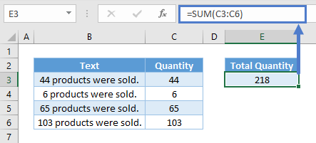
To overcome the issues above, you can use VALUE to convert from text to values.

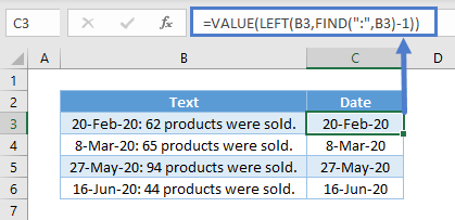
Extract Number from the Left of a String

Extract Number from the Left

We could combine LEFT, SUM, SUBSTITUTE with LEN as follows:

=LEFT(B2,SUM(LEN(B2)-LEN(SUBSTITUTE(B2,{"0","1","2","3","4","5","6","7","8","9"},""))))

Which would give us the following results:

Trim text to Nth words

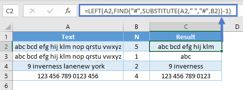
We could trim text to a number of words by combining SUBSTITUTE, FIND with LEFT as follows:

=LEFT(A2,FIND("#",SUBSTITUTE(A2," ","#",B2))-1)

Which would give us the following results:

Extract initials from Name

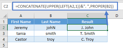
To extract initials from a name, we can combine CONCATENATE, UPPER, PROPER with LEFT as follows:

=CONCATENATE(UPPER(LEFT(A2,1))&". ",PROPER(B2,))

Which gives the following results.

Create Email Address Using First Name and Last Name

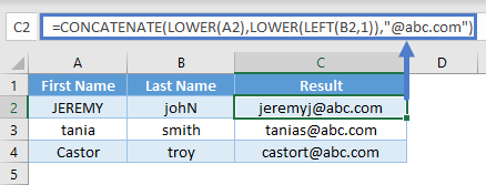
To create email addresses from first and last names, you can use a formula like this:

LEFT in Google Sheets

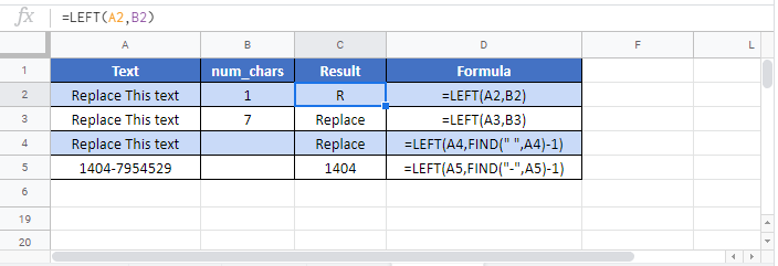
The LEFT Function works exactly the same in Google Sheets as in Excel:

LEFT Examples in VBA

You can also use the LEFT function in VBA. Type:

application.worksheetfunction.left(text,num_chars)