IMPT Function Examples – Excel, VBA, & Google Sheets

This tutorial demonstrates how to use the Excel IPMT Function in Excel to calculate the interest payment on a loan or an investment.

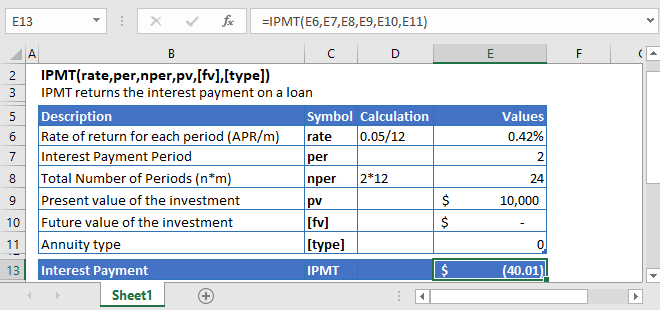
IPMT Function Overview

The IPMT Function Calculates the interest payment.

To use the IPMT Excel Worksheet Function, select a cell and type:

 

 

(Notice how the formula inputs appear)

IPMT Function Syntax and Inputs:

=IPMT(rate,nper,pv,[fv],[type])

rate – The interest rate for each period.

nper – The total number of payment periods.

pv – The present value of the investment that the future payments are worth now.

fv – OPTIONAL: The Future Value of the investment or loan at the end of the number of payment periods.

type – OPTIONAL: The type argument shows when the payments are made, either at the end of the period by 0 or at the start of the period by 1. Its default value is 0.

What is the Excel IPMT Function?

The Excel IPMT function calculates the interest payment for a given period based on the regular series of constant payments and a constant interest rate.

Calculate 2nd Interest Payment of a loan

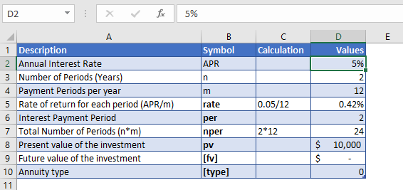
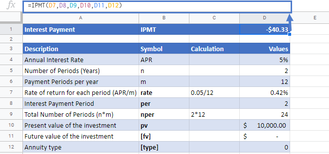
Let’s find out the second interest payment for a $10,000 investment that returns annually 5%. The investment is held for 2 years and the payments are made at the end of each month.

As the payments are made monthly, the annual interest rate is converted into monthly interest by

Monthly Interest Rate – 5% (annual interest rate) / 12 (months per year) = 0.42%

and the number of payments per period is converted into the monthly number of payments by

NPER – 2 (years) * 12 (months per year) = 24

The payments are made at the end of the month, so the value of [type] argument is

Type = 0

The Formula used for the calculation of principal payment is:

=IPMT(D7,D8,D9,D10,D11,D12)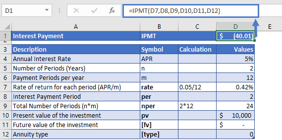

 

The monthly payment of the loan is

IPMT = -$40.01.

The result came in negative value because it shows that the cash is being paid out from the individual account.

Calculate 4th Interest Payment of an Investment

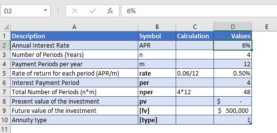
Now let’s calculate the 4^th interest payment of an investment, whose current value is $0. But it needs to be increased to $500,000 in the next four years. The annual interest rate is 6% and the payments are made at the start of each month.

As the payments are made monthly, the annual interest rate is converted into monthly interest by

Monthly Interest Rate – 4% (annual interest rate) / 12 (months per year) = 0.50%

and the number of payments per period is converted into the monthly number of payments by

NPER – 4 (years) * 12 (months per year) = 48

The payments are made at the start of the month, so the value of [type] argument is

Type = 1

The Formula used for the calculation of principal payment is:

=IPMT(D7,D8,D9,D10,D11,D12)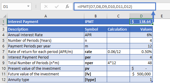

The interest payment for the fourth month is

IPMT = $138.64.

Additional Notes

Make sure the units of nper and rate are consistent, i.e. in case of monthly interest rate the number of periods of investment should also be in months.

In the Excel Financial Functions the cash outflows, such as deposits, are represented by negative numbers and the cash inflows, such as dividends, are represented by positive numbers.

#NUM! Error occurs when the value of the per argument is not between 1 and the value of nper argument.

#VALUE! Error occurs if any of the argument value is non-numeric.

Return to the List of all Functions in Excel

 

IPMT in Google Sheets

All of the above examples work exactly the same in Google Sheets as in Excel.

IPMT Examples in VBA

You can also use the IPMT function in VBA. Type:

application.worksheetfunction.ipmt(rate,nper,pv,fv,type)

For the function arguments (rate, etc.), you can either enter them directly into the function or define variables to use instead.