INDEX Function – Examples in Excel, VBA, & Google Sheets

This tutorial demonstrates how to use the INDEX Function in Excel and Google Sheets to return a value based on column and row references.

w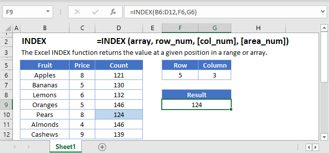

What is the INDEX function?

The INDEX Function returns a cell value from a list or table based on it’s column and row numbers.

Basic Example

We will start with a simple list of items (column A below). We want our formula to return the 3rd item from the list.

=INDEX(A2:A5, D1)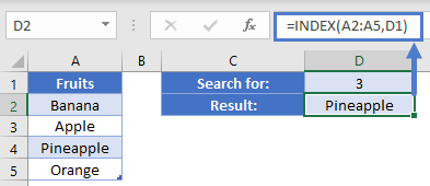

Within the INDEX Function, first we enter the array to search. Then we specify the row number of the item we want.

Table Example

Let’s build a multiplication table and demonstrate how to use the INDEX Function to return an item based on row / column index.

To get the result of 3 times 4 (and not just write the math equation), you could write a formula of

=INDEX(B2:E5, 3, 4)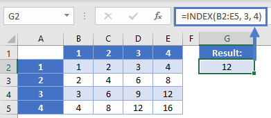

In this scenario, we’ve told the formula to go to the 3^rd row within the specified range, and the 4^th column. This is going to give a reference to cell E4, and we thus get a value of 12.

Table Example – Text

We can do the same with text values.

=INDEX(B2:D5, 3, 2)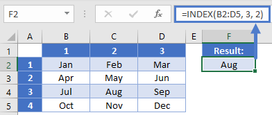

Here, our formula goes down to the 3^rd row (for the 3^rd quarter) and the 2^nd column. That returns a reference to C4 and the result of “Aug”.

MATCH with INDEX

The INDEX Function is often used in conjunction with the MATCH Function to create a lookup formula.

Let’s look at a grade book example where our teacher wants to be able to give a subject and student name and find the corresponding grade.

Our formula is.

=INDEX(B2:E5, MATCH(H1, A2:A5, 0), MATCH(H2, B1:E1, 0))

We’ve used two different MATCH function to return the relative position of each of our search terms. The first one is looking for the value of H1, “Reading”, in the range of A2:A5. Reading is the 3^rd item in the list. Our 2^nd MATCH is similarly looking for the value of “Bob” within the range B1:E1. Bob is the 2^nd item in this list. Thus, our formula will be evaluated like so:

=INDEX(B2:E5, MATCH(H1, A2:A5, 0), MATCH(H2, B1:E1, 0))
=INDEX(B2:E5, 3, 2)
=C4
=89

 

You can learn more about the INDEX / MATCH Formula by clicking the link.

 

INDEX in Google Sheets

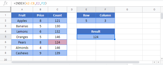
The INDEX Function works exactly the same in Google Sheets as in Excel:

 

INDEX Examples in VBA

You can also use the INDEX function in VBA. Type:

application.worksheetfunction.index(array,row_num,column_num)

For the function arguments (array, etc.), you can either enter them directly into the function, or define variables to use instead.

Assuming we have the following data in our worksheet

 

There are two tables defined in this example, one table on the left which is named Table2 and on the right Table3

We can use the INDEX function as following

WorksheetFunction.Index(Range("B2:F6"), 3, 3)

This will return 18 (Cell D4), because it is the cell located at the third row and third column cell in our defined range B2:F6

WorksheetFunction.Index(Range("Table2"), 2, 4)

This will return 51 (Cell E3), because it is the cell located at the second row and fourth column in Table2

We can also define more that one ranges, as following.Notice that we are using one more parameter this time (the last “1”), which defines the range from which the value should be returned

WorksheetFunction.Index(Range("B2:F6,I4:M8"), 2, 5, 1)

This will return 36 (Cell F3), because it is the cell located at the second row and fifth column in our first defined range, which is Table2

 WorksheetFunction.Index(Range("B2:F6,I2:M6"), 4, 3, 2)

This will return 115 (Cell K5), because it is the cell located at the fourth row and third column in our second defined range, which is I2:M6