FV Function – Future Value in Excel, VBA, Google Sheets

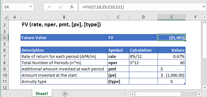
This tutorial demonstrates how to use the FV Function in Excel to calculate the future value of an investment.

What Is Future Value?

It’s the value of the investment at a particular date in the future that is equivalent in value to a specified sum today.

The Future Value is calculated in two ways:

1. Future Value Using Simple Annual Interest Rate is calculated as:

2. Future Value Using Compounded Annual interest Rate is calculated as:

Where:

I = Invested Amount

R = Interest Rate

T = Number of periods

What Is Excel FV Function?

FV is used to determine how much the investment will be worth at the end of the given period if there are regular and constant deposits at constant interest rates.

Calculate Future Value of Savings

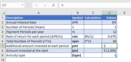
Suppose, we deposited $1,000 for 4 years into a savings account. The interest we get from this was 8% annually, which was compounded monthly and with no additional payments.

The annual interest rate is converted into monthly interest as

Monthly Interest Rate – 8% (annual interest rate) / 12 (months per year) = 0.67%

and the number of payments per period is converted into the monthly number of payments as

NPER – 5 (years) * 12 (months per year) = 60

No regular payments are being made, so the value of pmt argument is

PMT = 0

The formula used for the calculation is:

=FV(D7,D8,D9,D10,D11)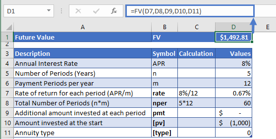

The Future Value of the investment is

FV = $1,492.81

Calculate Future Value of an Investment

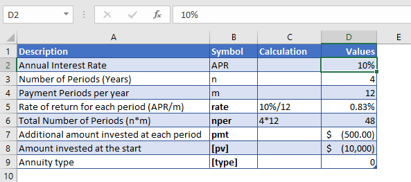
Let’s take a look at another example, where $10,000 has been invested at 10% compounded monthly for 4 years. And on top of the initial deposit, an additional amount of $500 are planned to be invested each month for the next four years. So the future value of the total savings would be calculated with the help of excel FV Formula.

As the payments are made monthly, the annual interest rate is converted into monthly interest by

Monthly Interest Rate – 10% (annual interest rate) / 12 (months per year) = 0.83%

and the number of payments per period is converted into the monthly number of payments by

NPER – 4 (years) * 12 (months per year) = 48

The formula used for the calculation is:

=FV(D7,D8,D9,D10,D11)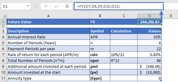

So, the accumulated amount at the end of the 4^th year would be

FV = $44,206.83

FV in Google Sheets

All of the above examples work exactly the same in Google Sheets as in Excel.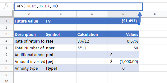

Additional Notes

Use the FV Function to calculate the Future Value of an investment.
Investopedia defines future value as: The value of an asset or cash at a specified date in the future that is equivalent to a specified sum today.

Make sure the units of nper and rate are consistent, i.e. in case of monthly interest rate the number of periods of investment should also be in months.

In the Financial Functions the cash outflows, such as deposits, are represented by negative numbers and the cash inflows, such as dividends, are represented by positive numbers.

FV Examples in VBA

You can also use the FV function in VBA. Type:

application.worksheetfunction.fv(rate,nper,pmt,pv,type)

For the function arguments (rate, etc.), you can either enter them directly into the function or define variables to use instead.