FIND Function Examples In Excel, VBA, & Google Sheets

This tutorial demonstrates how to use the FIND Function in Excel and Google Sheets to find text within text.

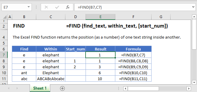
What Is the FIND Function?

The Excel FIND Function tries to find string of text within another text string. If it finds it, FIND returns the numerical position of that string.

Note: FIND is case-sensitive. So, “text” will NOT match “TEXT”. For case-insensitive searches, use the SEARCH Function.

 

How to Use the FIND Function

To use the Excel FIND Function, type the following:

=FIND("e", "elephant")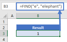

In this case, Excel will return the number 1, because “e” is the first character in the string “elephant”.

Let’s take a look at some more examples:

Start Number (start_num)

The start number tells FIND what numerical position in the string to start looking from. If you don’t define it, FIND will start from the beginning of the string.

=FIND(B3,C3)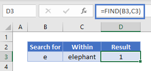

 

Now let’s try defining a start number of 2. Here, we see that FIND returns 3. Because it starts looking from the second character, it misses the first “e” and finds the second:

=FIND(B3,C3,D3)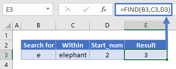

Start Number (start_num) Errors

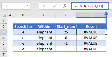
If you want to use a start number, it must:

• be a whole number
• be a positive number
• be smaller than the length of the string you are looking in
• not refer to a blank cell, if you define it as a cell reference

Otherwise, FIND will return a #VALUE! error as shown below:

Unsuccessful Searches Return a #VALUE! Error

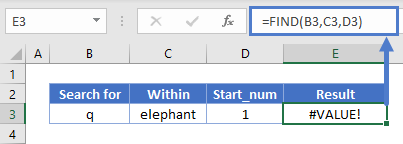
If FIND does not locate the string you’re looking for, it will return a value error:

FIND is Case-Sensitive

In the example below, we’re searching for “abc”. FIND returns 10 because it is case-sensitive – it ignores “ABC” and the other variations:

 

FIND Does Not Accept Wildcards

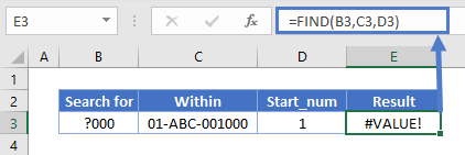
You cannot use wildcards with FIND. Below, we’re looking for “?000”. In a wildcard search, this would mean “any character followed by three zeroes”. But FIND takes this literally to mean “a question mark followed by three zeroes”:

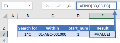
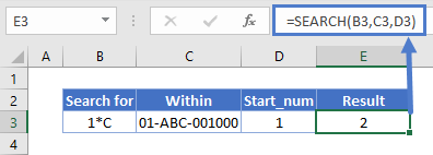
The same applies to the asterisk wildcard:

 

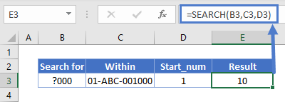
Instead, to search text with wildcards, you can use the SEARCH Function:

How to Split First and Last Names from a Cell with FIND

If your spreadsheet has a list of names with both the first and last names in the same cell, you might want to split them out to make sorting easier. FIND can do that for you – with a little help from some other functions.

Getting the First Name

The LEFT Function returns a given number of characters from a string, starting from the left.

We can use it to get the first name, but since names are different lengths, how do we know how many characters to return?

Easy – we just use FIND to return the position of the space between the first and last name, subtract 1 from that, and that’s how many characters we tell LEFT to give us.

The formula looks like this:

=LEFT(B3,FIND(“ “,B3)-1)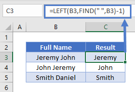

Getting the Last Name

The RIGHT Function returns a given number of characters from a string, starting from the right.

We have the same problem here as with the first name, but the solution is different, because we have to get the number of characters between the space and the right edge of the string, not the left.

To get that, we use FIND to tell us where the space is, and then subtract that number from the total number of characters in the string, which the LEN Function can give us.

The formula looks like this:

=RIGHT(B3,LEN(B3)-FIND(" ",B3))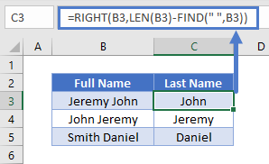

If the name contains a middle name, note that it will be split into the last name cell.

Finding the nth Character in a String

As noted above, FIND returns the position of the first match it finds. But what if you want to find the second occurrence of a particular character, or the third, or fourth?

This is possible with FIND, but we’ll need to combine it with a couple of other functions: CHAR and SUBSTITUTE.

Here’s how it works:

• CHAR returns a character based on its ASCII code. For example, =CHAR(134) returns the dagger symbol.
• SUBSTITUTE goes through a string and lets you swap out a character for any other one.
• With SUBSTITUTE you can define an instance number, meaning it can swap the nth occurrence of a given string for anything else.
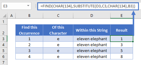
• So, the idea is, we take our string, use SUBSTITUTE to swap the instance of the character we want to find for something else. We’ll use CHAR to swap it for something that is unlikely to be found in the string, then use FIND to locate that obscure substitute.

The formula looks like this:

=FIND(CHAR(134),SUBSTITUTE(D3,C3,CHAR(134),B3))

And here’s how it works in practice:

FIND Vs SEARCH

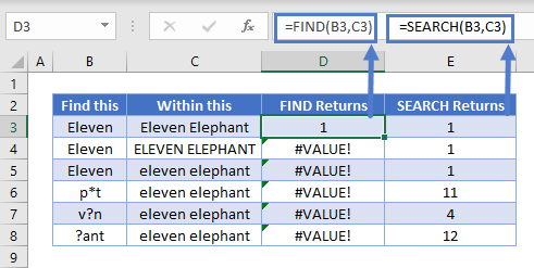
FIND and SEARCH are very similar – they both return the position of a given character or substring within a string. However, there are some differences:

• FIND is case sensitive but SEARCH is not
• FIND does not allow wildcards, but SEARCH does

You can see a few examples of these differences below:

FIND in Google Sheets

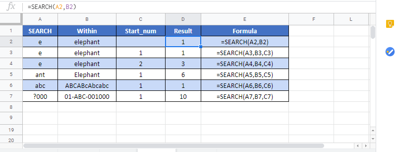
The FIND Function works exactly the same in Google Sheets as in Excel:

Additional Notes

The FIND Function is case-sensitive.

The FIND Function does not support wildcards.

Use the SEARCH Function to use wildcards and for non case-sensitive searches.

FIND Examples in VBA

You can also use the FIND function in VBA. Type:

application.worksheetfunction.find(find_text,within_text,start_num)

For the function arguments (find_text, etc.), you can either enter them directly into the function, or define variables to use instead.