DSUM Function – Examples in Excel, VBA, Google Sheets

This tutorial demonstrates how to use the DSUM Function in Excel to sum records in a database.

What is the DSUM Function?

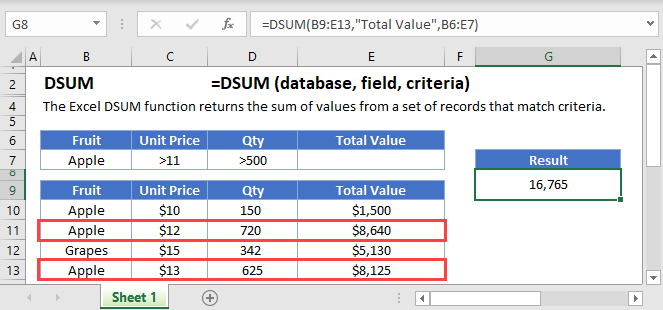
DSUM is one of Excel’s database functions. It returns the sum of a column in a database, after applying a range of filters to the data.

Note that when we say “database” in this context, we just mean a table of data in Excel, that has been organized with column headers.

How to Use the DSUM Function

To use the Excel DSUM Function, type the following:

=DSUM(B7:F19,"Oscars won",B3:F4)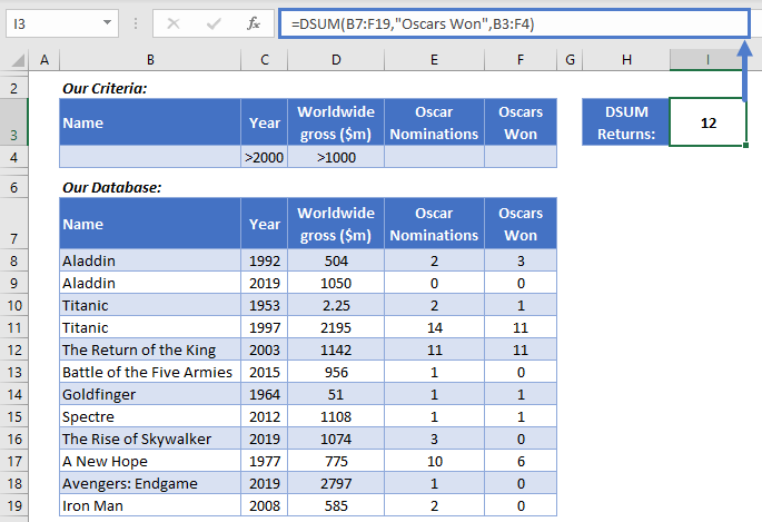

In this example, we have a database with some movie data. We want to know how many Oscars were won by movies released after the year 2000, that grossed over $1bn. DSUM can get that information for us.

Here’s how DSUM works:

• The first argument is the database, cells B7:F19. Note: you must include your column headers in this range.
• The second argument is the column we want to sum – Oscars Won. You can refer to columns by their name in quotations, or by their numerical position (so we could also just put 5 here).
• In the third argument we define the filters we want DSUM to apply before calculating the sum. These are in B3:F4.

Take a closer look at the filters we’ve defined in B3:F4. We’ve got the same headers as the database, and we’ve defined two criteria: a “Year” greater than 2000, and a “Worldwide Gross ($m)” greater than 1000.

DSUM correctly returns 12 Oscars. Two movies meet these criteria: The Return of the King, doing the monarch’s share of the work with 11 Oscars, and Spectre, which adds 1 more to the total.

DSUM Sums Numerical Values Only

DSUM will only include rows with numerical data, and will ignore text. For example, if we try summing the “Name” column, DSUM will return 0, because it doesn’t find any numerical data to sum.

=DSUM(B7:F19,"Name",B3:F4)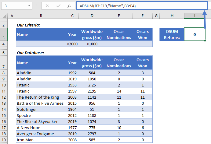

Criteria

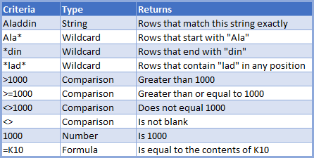
DSUM enables you to use a range of different criteria when filtering your data. Here are a few common examples:

Multiple Criteria Rows

When you create your criteria table, you can use more than one row if you need to.

If you do use more than one row, DSUM will use “OR” logic – it will include data that matches any of your criteria rows.

Here’s an example:

=DSUM(B8:F20, 5,B3:C5)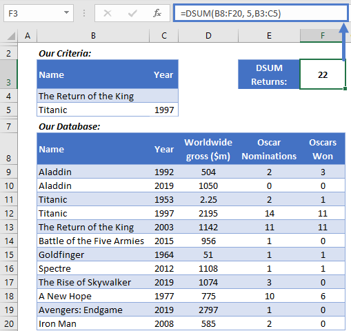

We want to know how many Oscars 1997’s Titanic and 2003’s The Return of the King won in total. Since there are two movies called “Titanic” in the database, we’ve also specified the year in our criteria table.

Note also, we’ve only used the two columns we want to filter on in our criteria table – you don’t need to include them all.

DSUM returns 22 – 11 for each movie.

Use SUM When You Don’t Need to Filter the Data

DSUM is a powerful tool when you need to filter the data in complex ways. But if you don’t need to use filters, use SUM instead.

You use SUM like this:

=SUM(C3:C14)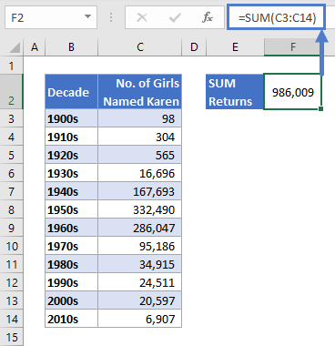

As you can see here, with SUM you simply define the range containing your data, and it will return the sum of any numerical cells within that range.

Learn more on the SUM Function tutorial.

DSUM in Google Sheets

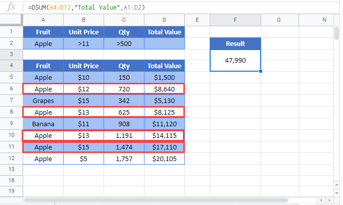
The DSUM Function works exactly the same in Google Sheets as in Excel:

DSUM Examples in VBA

You can also use the DSUM function in VBA. Type:

application.worksheetfunction.dsum(database,field,criteria)