COLUMN Function Examples – Excel & Google Sheets

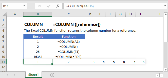
This Tutorial demonstrates how to use the Excel COLUMN Function in Excel to look up the column number of a cell.

COLUMN Function – Single Cell

The COLUMN Function returns the column number of the given cell reference. 

=COLUMN(U8)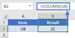

COLUMN Function with no Reference

If no cell reference is provided, the COLUMN Function will return the column number where the formula is entered.

=COLUMN()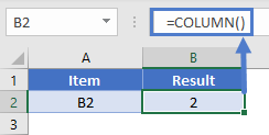

COLUMN Function with a Range

You can also input entire ranges of cells into the COLUMN Function. When doing so, the COLUMN Function behaves differently in Excel 2019 (or earlier) vs. Excel 365 or newer version of Excel.

Excel 2019 or older

In previous versions of Excel, the COLUMN Function returns an array containing the column values of all the cells in the range, but only displays the first result in the cell.

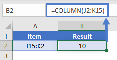
If you click the cell containing the formula and press F9, all the results are displayed in curly brackets as an array.

={10,11}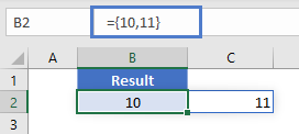

Excel 365

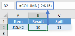
However, Excel 365 (and newer versions of Excel, presumably) comes with a spill range feature. Here, the COLUMN Function will return the columns of all cells in the range, “spilled” into the next cells.

Column Letter Instead of Number

What if you want the column letter of a cell reference, instead of a column number? Use this complicated formula instead:

=SUBSTITUTE(ADDRESS(1,COLUMN(),4),"1","")

This formula calculates the column number with the COLUMN Function and calculates the address of a cell in row 1 of that column using the ADDRESS Function. Then it uses the SUBSTITUTE Function to remove the row number (1), so all that remains is the column letter.

COLUMN Function in Google Sheets

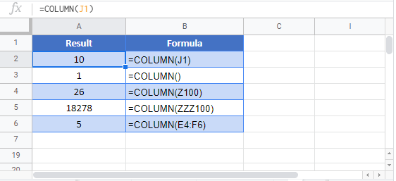
The COLUMN Function works exactly the same in Google Sheets as in Excel: