CELL Function Examples – Excel & Google Sheets

This Tutorial demonstrates how to use the Excel CELL Function in Excel to get information about a cell.

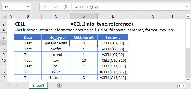
CELL Function Overview

The CELL Function Returns information about a cell. Color, filename, contents, format, row, etc.

To use the CELL Excel Worksheet Function, select a cell and type:

(Notice how the formula inputs appear)

CELL function Syntax and inputs:

=CELL(info_type,reference)

info_type – Text indicating what cell information you would like to return.

reference – The cell reference that you want information about.

How to use the CELL Function in Excel

The CELL Function returns information about the formatting, location, or contents of cell.

=CELL(D3,$B$3)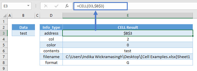

As seen above, the CELL Function returns all kinds of information from cell B3.

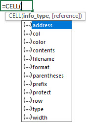
If you type =CELL(, you will be able to see 12 different types of information to retrieve.

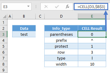
Here are additional outputs of the CELL Function:

Overall View of Info_types

Some of the info_types are pretty straightforward and retrieves what you asked for, while the rest will be explained in the next few sections because of the complexity.

Info_type	What it retrieves?
“address”	The cell reference/address.
“col”	The column number.
“color”	*
“contents”	The value itself or result of the formula.
“filename”	The full path, filename, and extension in square brackets, and sheet name.
“format”	*
“parentheses”	*
“prefix”	*
“protect”	*
“row”	The row number.
“type”	*
“width”	The column width rounded to the nearest integer.

* Explained in the next few sections.

Color Info_type

Color will show all results as 0 unless the cell is formatted with color for negative values. The latter will show as 1.

=CELL("color",B3)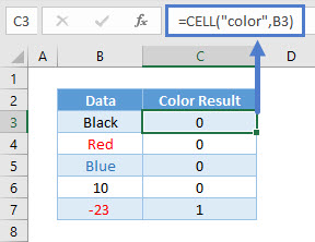

Format Info_type

Format shows the number format of the cell, but it might not be what you expect.

=CELL("format",B3)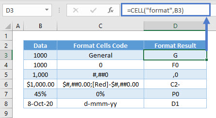

There are many kinds of different variations with formatting, but here are some guidelines to figure it out:

• “G” is for General, “C” for Currency, “P” for Percentage, “S” for Scientific (not shown above), “D” for Date.
• If the digits are with numbers, currencies, and percentages; it represents the decimal places. Eg. “F0” means 0 decimals in cell D4, and “C2-” means 2 decimals in cell D6. “D1” in cell D8 is simply a type of date format (there are D1 to D9 for different kinds of date and time formats).
• A comma at the beginning is for thousand separators (“,0” in cell D5 for eg).
• A minus sign is for formatting negative values with a color (“C2-” in cell D6 for eg).

Here are other examples of date formats and for scientific.

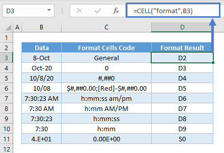
Parentheses Info_type

Parentheses shows 1 if the cell is formatted with parentheses (either or both positive and negative). Otherwise, it shows 0.

=CELL("parentheses",B3)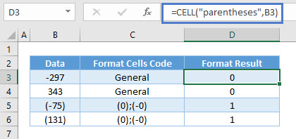

Prefix Info_type

Prefix results in various symbols depending on how the text is aligned in the cell.

=CELL("prefix",B3)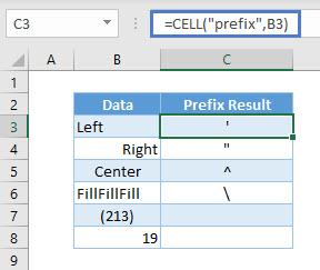

As seen above, a left alignment of the text is a single quote in cell C3.
A right alignment of the text shows double quotes in cell C4.
A center alignment of the text shows caret in cell C5.
A fill alignment of the text shows backslash in cell C6.
Numbers (cell C7 and C8) show as blank regardless of alignment.

Protect Info_type

Protect results in 1 if the cell is locked, and 0 if it’s unlocked.

=CELL("protect",B3)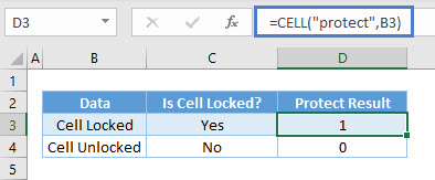

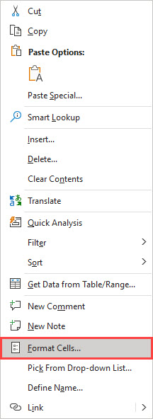
Do note that all cells are locked by default. That is why you can’t edit any cells after you protect it. To unlock it, right-click on a cell and choose Format Cells.

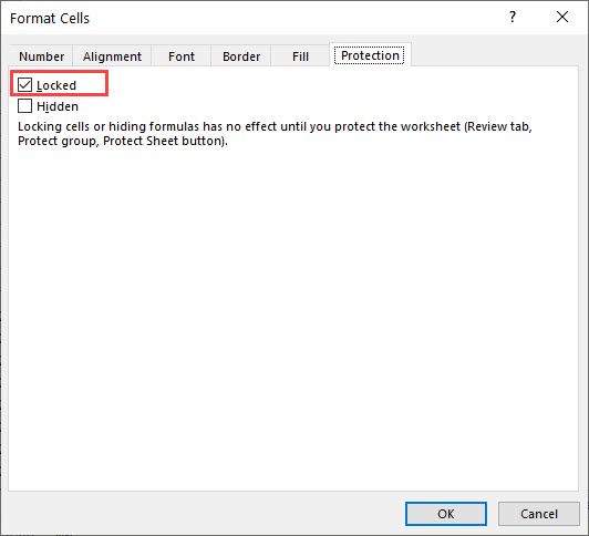
Go to the Protection tab and you can uncheck “Locked” to unlock the cell.

Type Info_type

Type results in three different alphabets dependent on the data type in the cell.

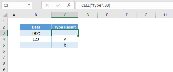
“l” stands for label in cell C3.
“v” stands for value in cell C4.
“b” stands for blank in cell C5.

Create Hyperlink to Lookup Using Address

You can use the CELL Function along with HYPERLINK and INDEX / MATCH to hyperlink to a lookup result:

=HYPERLINK("#"&CELL("address",INDEX(C3:C6,MATCH("mango",B3:B6,0))),INDEX(C3:C6,MATCH("mango",B3:B6,0)))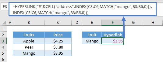

The INDEX and MATCH formula retrieves the price of Mango in cell C5: $3.95. The CELL Function, with “address” returns the cell location. The HYPERLINK function then creates the hyperlink.

Retrieve File Path

To retrieve the file path where the particular file is stored, you can use:

=LEFT(CELL("filename"),FIND("[",CELL("filename"))-1)

Since the filename will be the same using any cell reference, you can omit it. Use FIND function to obtain the position where “[“ starts and minus 1 to allow LEFT function to retrieve the characters before that.

Retrieve File Name

To retrieve the file name, you can use:

=MID(CELL("filename"),FIND("[",CELL("filename"))+1,FIND("]",CELL("filename"))-FIND("[",CELL("filename"))-1)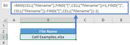

This uses a similar concept as above where FIND function obtains the position where “[“ starts and retrieves the characters after that. To know how many characters to extract, it uses the position of “]” minus “[“ and minus 1 as it includes the position of “]”.

Retrieve Sheet Name

To retrieve the sheet name, you can use:

=MID(CELL("filename"),FIND("]",CELL("filename"))+1,LEN(CELL("filename")))

Again, it’s similar to the above where FIND function obtains the position where “]“ starts and retrieves the characters after that. To know how many characters to extract, it uses the total length of what “filename” info_type returns.

CELL Function in Google Sheets

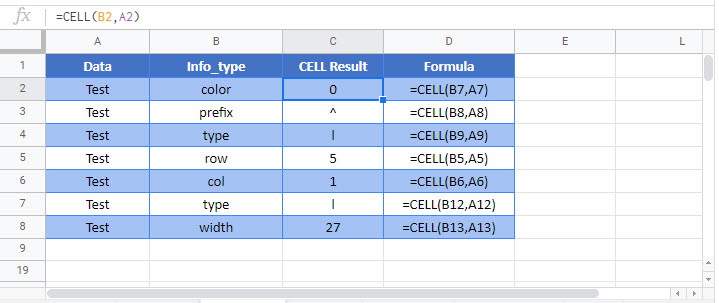
The CELL function works similarly in Google Sheets. It just doesn’t have the full range of info_type. It only includes “address”, “col”, “color”, “contents”, “prefix”, “row”, “type”, and “width”.

 

Additional Notes

The CELL Function returns information about a cell. The information that can be returned relates to cell location, formatting and contents.

Enter the type of information you want then enter the cell reference for the cell you want information about.

Return to the List of all Functions in Excel