VLOOKUP – Fix #N/A Error – Excel & Google Sheets

This tutorial will demonstrate how to handle #N/A Errors when performing VLOOKUPs in Excel and Google Sheets. If your version of Excel supports XLOOKUP, we recommend using the XLOOKUP Function instead.

VLOOKUP: #N/A Error-Handling

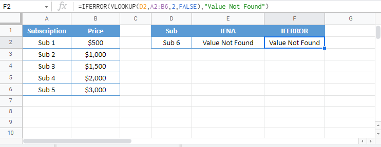
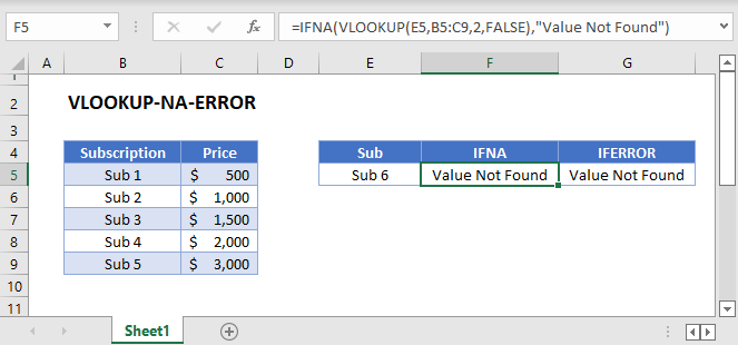
The VLOOKUP Function returns the #N/A Error when it fails to find a match. Instead, you may want to return some other value if a match is not found. There are two functions that we can use to replace this error with a customized value: IFNA and IFERROR.

VLOOKUP with IFNA

In this example, we will replace the #N/A Error with the text “Value Not Found” using the IFNA Function.

=IFNA(VLOOKUP(E3,B3:C7,2,FALSE),"Value Not Found")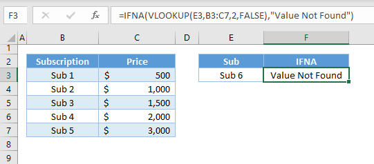

Let’s walk through the formula above:

VLOOKUP Function

The VLOOKUP Function searches for the lookup value (e.g., Sub), and if it doesn’t find a match, it will return the #N/A Error.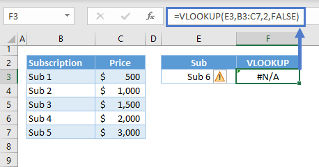

Note: The VLOOKUP Function searches for the lookup value from the first column of the table and returns the corresponding value from the column defined by the col_index_num.

 

IFNA Function

The IFNA Function looks for the #N/A Error. If found, the specified value (e.g., “Value Not Found”) is returned.

=IFERROR(F3,"Value Not Found")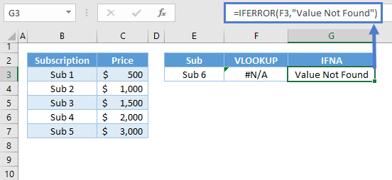

 

Combining the functions together gives us our original formula:

=IFNA(VLOOKUP(E3,B3:C7,2,FALSE),"Value Not Found")

Instead of a text, we can also replace the #N/A Error with a numerical value like 0:

=IFNA(VLOOKUP(E3,B3:C7,2,FALSE),0)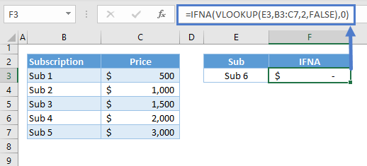

 

VLOOKUP with IFERROR

The IFNA and IFERROR functions work exactly the same way, except the IFERROR Function handles all types of errors (e.g., #N/A, #REF!, #VALUE!).

=IFERROR(VLOOKUP(E3,B3:C7,2,FALSE),"Value Not Found")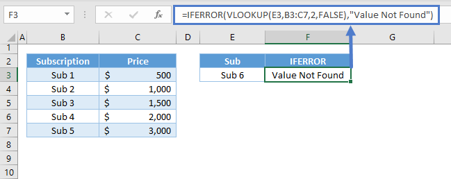

We recommend using the IFNA function instead of the more common IFERROR because IFNA will only replace the #N/A error. Using IFNA will make sure you don’t miss other important errors.

 

VLOOKUP: Multiple Sheets at Once

Instead of a customized value, we can nest another VLOOKUP Function inside IFNA/IFERROR if we want to perform a VLOOKUP on multiple sheets at once.

VLOOKUP with IFNA: Two Sheets at Once

=IFNA(VLOOKUP(E3,B3:C7,2,FALSE),VLOOKUP(E3,'2 Sheets - Data 2'!B3:C7,2,FALSE))

 

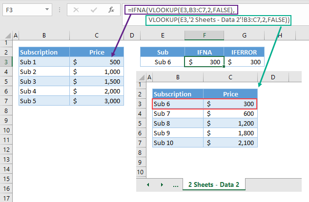
Let’s walk through the formula above:

VLOOKUP Function

We need to perform a VLOOKUP on each sheet. This will perform the lookup on the first sheet:

=VLOOKUP(E3,B3:C7,2,FALSE)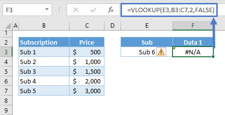

 

This will perform the lookup on the second sheet:

=VLOOKUP(E3,'2 Sheets - Data 2'!B3:C7,2,FALSE)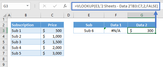

 

IFNA Function

Then we use the IFNA Function to return the result of the second VLOOKUP, if the first VLOOKUP does not find a match.

=IFNA(F3,G3)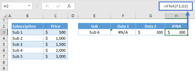

Combining all the functions gives our original formula:

=IFNA(VLOOKUP(E3,B3:C7,2,FALSE),VLOOKUP(E3,'2 Sheets - Data 2'!B3:C7,2,FALSE))

 

VLOOKUP with IFNA/IFERROR in Google Sheets

The IFNA-VLOOKUP and IFERROR-VLOOKUP work the same way in Google Sheets as in Excel.

=IFNA(VLOOKUP(E3,B3:C7,2,FALSE),"Value not Found")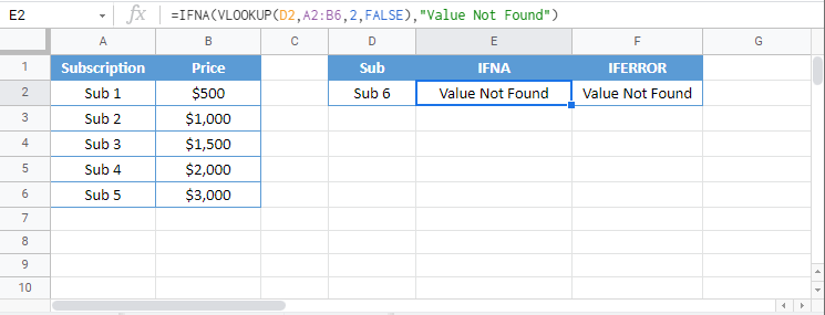

 

=IFERROR(VLOOKUP(E3,B3:C7,2,FALSE),"Value not Found")