VLOOKUP & INDIRECT – Dynamic Range – Excel & Google Sheets

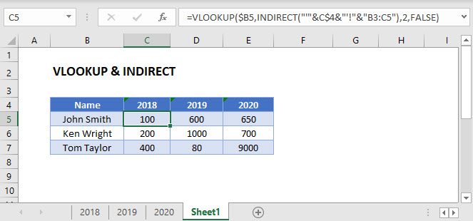
This tutorial will demonstrate how to use the INDIRECT Function to define the lookup range in Excel and Google Sheets.

INDIRECT & VLOOKUP

You may need to perform a VLOOKUP on multiple ranges at once, dependent on certain cell values. If so, one option is the INDIRECT Function, which can be used to define a lookup range, or even create a dynamic reference to multiple sheets.

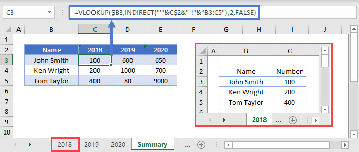
=VLOOKUP($B3,INDIRECT("'"&C$2&"'!"&"B3:C5"),2,FALSE)

Here we have data in range B3:C5 on every sheet. Instead of writing a VLOOKUP formula for each sheet, we can dynamically refer to the sheets with the INDIRECT Function.

INDIRECT – Dynamic Lookup Range

We need the lookup range for C3 to look like:

'2018!'B3:C5

So all we need to do is write a formula that will generate that range within the INDIRECT Function:

"'"&C$2&"'!"&"B3:C5"

We use (&) to merge together the text along with the partially-locked cell reference containing the year (C$2). Then when the formula is copied across the range, the INDIRECT function will output the necessary sheet for each column.

CHOOSE & VLOOKUP

The INDIRECT Function is “volatile.” It recalculates every time Excel does, and that can cause your workbook to calculate slowly.

Instead, in this case, the CHOOSE Function might be a better alternative. The CHOOSE Function let’s you “choose” what to output from a list.

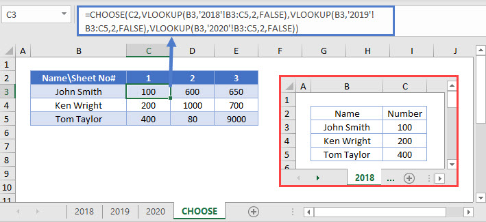
=CHOOSE(C2,VLOOKUP(B3,'2018'!B3:C5,2,FALSE),VLOOKUP(B3,'2019'!B3:C5,2,FALSE),VLOOKUP(B3,'2020'!B3:C5,2,FALSE))

In this example, the list in the CHOOSE Function is each possible VLOOKUP formula. Each range is hard-coded, and each cell references all three sheets. The index value in Row 2 tells the function which element of the list to use, i.e. which sheet to perform the lookup on.

VLOOKUP & INDIRECT in Google Sheets

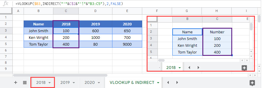
These formulas work the same in Google Sheets as in Excel.