Case Sensitive VLOOKUP in Excel & Google Sheets

This tutorial will demonstrate how to perform a case-sensitive VLOOKUP in Excel using two different methods and Google Sheets using one method.

Case-Sensitive VLOOKUP with Helper Column

VLOOKUP Function

The VLOOKUP Function is used to look up an approximate or exact match for a value in the leftmost column of a range and returns the corresponding value from another column. By default, VLOOKUP will only work for non-case-sensitive values like so:

=VLOOKUP($E$2,$B$2:$C$4,2,0)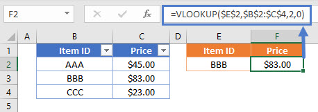

Case-Sensitive VLOOKUP

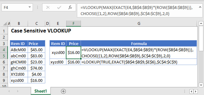
By combining VLOOKUP, EXACT, MAX and ROW, we can create a case-sensitive VLOOKUP formula that returns the corresponding value for our case-sensitive VLOOKUP. Let’s walk through an example.

We have a list of items and their corresponding prices (notice that Item ID is case-sensitive unique):

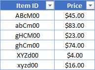
Supposed we are asked to get the price for an item using its Item ID like so:

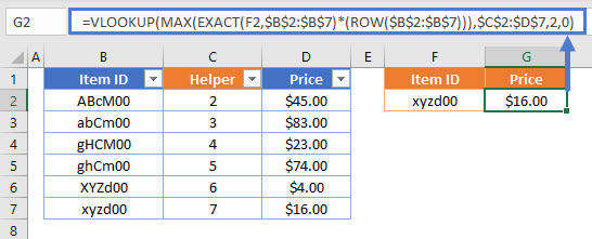
To accomplish this, we fist need to create a helper column using ROW:

=ROW()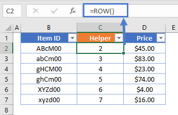

=ROW() click and drag (or double-click) to prefill all rows in the range

Next, combine VLOOKUP, MAX, EXACT and ROW in a formula like so:

=VLOOKUP(MAX(EXACT(<lookup value>,<lookup range>)*(ROW(<lookup range>))),
<helper range>,<match range position>,0)

=VLOOKUP(MAX(EXACT(E2,$B$2:$B$7)*(ROW($B$2:$B$7))),$C$2:$D$7,2,0)

How does the formula work?

1. The EXACT function checks the Item ID in E2 (lookup value) against the values in B2:B7 (lookup range) and returns an array of TRUE where there is an exact match or FLASEs in an array {FLASE, FLASE, FLASE, FLASE, FLASE, TRUE}.
2. This array is then multiplied by the ROW array {2, 3, 4, 5, 6, 7} (note that this matches our helper column).
3. The MAX function returns the maximum value from the resulting array {0,0,0,0,0,7}, which is 7 in our example.
4. Then we use the result as our lookup value in a VLOOKUP and choose our helper column as the lookup range. In our example, the formula returns the matching value of $16.00.

Method 2 – case-sensitive VLOOKUP with “virtual” helper column

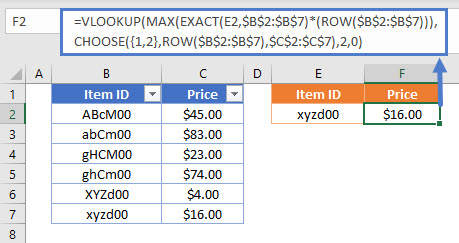
This method uses the same logic as the first method, but eliminates the need for creating a helper column and instead uses CHOOSE and ROW to create a “virtual” helper column like so:

=VLOOKUP(MAX(EXACT(<lookup value>,<lookup range>)*(ROW(<lookup range>))), 
CHOOSE({1,2}, ROW(<lookup range>), <match range>), <match range position>,0)

=VLOOKUP(MAX(EXACT(D2,$B$2:$B$7)*(ROW($B$2:$B$7))),CHOOSE({1,2},ROW($B$2:$B$7),$C$2:$C$7),2,0)

How does the formula work?

1. The first part of the formula works the same way as the first method.
2. Combining CHOOSE and ROW returns an array with two columns, one for the row number and another for the price. The array is separated by a semicolon to represent the next row and a comma for the next column like so: {2,45; 3,83; 4,23; 5,74; 6,4; 7,16}.
3. We can then use the result from the first part of the formula in a VLOOKUP to find the corresponding value from our CHOOSE and ROW array.

Case Sensitive VLOOKUP in Google Sheets

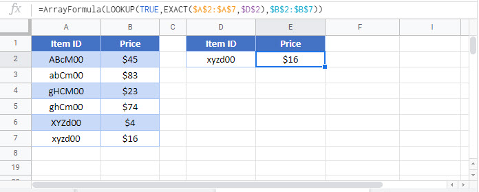
To perform a case-sensitive VLOOKUP in Google Sheets, use this method: