Sum if Across Multiple Sheets – Excel & Google Sheets

This tutorial will demonstrate how to use the SUMPRODUCT and SUMIFS Functions to sum data that meets certain criteria across multiple sheets in Excel and Google Sheets.

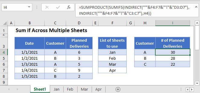
Regular Sum Across Multiple Sheets

Sometimes your data might span several worksheets in an Excel file. This is common for data that is collected periodically. Each sheet in a workbook might contain data for a set time period. We want a formula that sums data contained in two or more sheets.

The SUM Function allows you to easily sum data across multiple sheets using a 3D Reference:

=SUM(Sheet1:Sheet2!A1)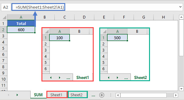

However, this is not possible with the SUMIFS Function. Instead we must use a more complicated formula.

Sum if Across Multiple Sheets

This example will sum the Number of Planned Deliveries for each Customer over multiple worksheets, each holding data relating to a different month, by using the SUMIFS, SUMPRODUCT, and INDIRECT Functions:

=SUMPRODUCT(SUMIFS(INDIRECT("'"&F3:F6&"'!"&"D3:D7"),INDIRECT("'"&F3:F6&"'!"&"C3:C7"),H3))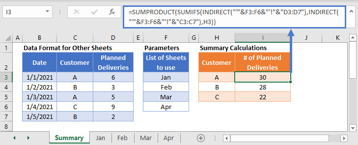

Let’s walk through this formula.

Step 1: Create a SUMIFS Formula for 1 Input Sheet Only:

We use the SUMIFS Function to sum the Number of Planned Deliveries by Customer for a single input data sheet:

=SUMIFS(D3:D7,C3:C7,H3)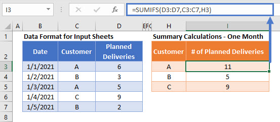

Step 2: Add a Sheet Reference to the Formula

We keep the formula result the same, but we specify that the input data is in the sheet called ‘Step 2’

=SUMIFS('Step 2'!D3:D7,'Step 2'!C3:C7,H3)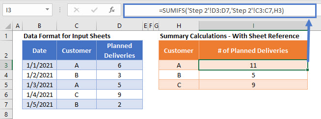

Step 3 : Nest Inside a SUMPRODUCT Function

To prepare the formula to perform SUMIFS calculations over multiple sheets and then to sum the results together, we add a SUMPRODUCT Function around the formula

=SUMPRODUCT(SUMIFS('Step 3'!D3:D7,'Step 3'!C3:C7,H3))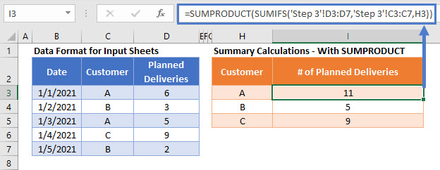

Using the SUMIFS Function on one sheet yields a single value. Across multiple sheets, the SUMIFS function outputs an array of values (one for each worksheet). We use the SUMPRODUCT Function to total the values in this array.

Step 4: Replace the Sheet Reference with a List of Sheet Names

We wish to replace the Sheet Name part of the formula with a data list containing the values: Jan, Feb, Mar, and Apr. This list is stored in the cells F3:F6.

The INDIRECT Function to ensures that the text list showing Sheet Names is treated as part of a valid cell reference in the SUMIFS Function.

=SUMPRODUCT(SUMIFS(INDIRECT("'"&F3:F6&"'!"&"D3:D7"),INDIRECT("'"&F3:F6&"'!"&"C3:C7"),H3))

In this formula, the previously written range reference:

'Step 3'!D3:D7

Is replaced by:

INDIRECT("'"&F3:F6&"'!"&"D3:D7")

The quotation marks makes the formula difficult to read, so here it is shown with added spaces:

INDIRECT ( " ' " & F3:F6 & " ' ! " & "D3:D7" )

Using this way of referencing a list of cells also allows us to summarize data from multiple sheets which do not follow a numerical list style. A standard 3D reference would require the sheet names to be in the style: Input1, Input2, Input3, etc., but the example above allows you to use a list of any Sheet Names and to have them referenced in a separate cell.

Locking Cell References

To make our formulas easier to read, we’ve shown the formulas without locked cell references:

=SUMPRODUCT(SUMIFS(INDIRECT("'"&F3:F6&"'!"&"D3:D7"),INDIRECT("'"&F3:F6&"'!"&"C3:C7"),H3))

But these formulas will not work properly when copy and pasted elsewhere in your file. Instead, you should use locked cell references like this:

=SUMPRODUCT(SUMIFS(INDIRECT("'"&$F$3:$F$6&"'!"&"D3:D7"),INDIRECT("'"&$F$3:$F$6&"'!"&"C3:C7"),H3))

Read our article on Locking Cell References to learn more.

Sum If Across Multiple Sheets in Google Sheets

Using the INDIRECT Function to reference a list of sheets in a SUMPRODUCT and SUMIFS Function is not currently possible in Google Sheets.

Instead, separate SUMIFS calculations can be made for each input sheet and the results added together:

=SUMIFS(Jan!D3:D7,Jan!C3:C7,H3)
+SUMIFS(Feb!D3:D7,Feb!C3:C7,H3)
+SUMIFS(Mar!D3:D7,Mar!C3:C7,H3)
+SUMIFS(Apr!D3:D7,Apr!C3:C7,H3)