Sum If By Month – Excel & Google Sheets

This tutorial will demonstrate how to use the SUMIFS Function to sum data corresponding to specific months in Excel and Google Sheets.

 

Sum if by Month

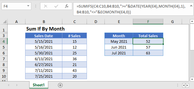
First, we will demonstrate how to sum data corresponding to dates that fall in a specific month and year.

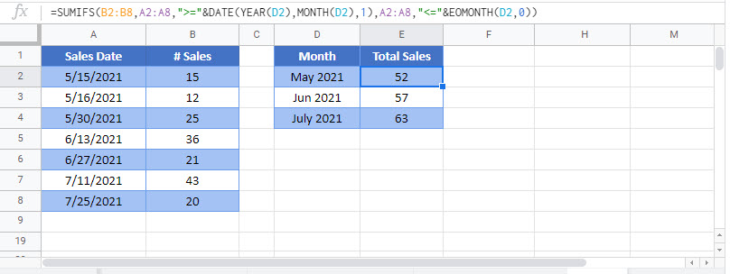
We can use the SUMIFS Function, along with the DATE, YEAR, MONTH, and EOMONTH Functions to sum the Number of Sales within each Month.

=SUMIFS(C3:C9,B3:B9,">="&DATE(YEAR(E3),MONTH(E3),1),B3:B9,"<="&EOMONTH(E3,0))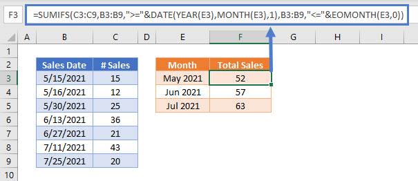

To build the formula above, we start by defining the date range for each month. We use the DATE Function to define the first day of the month (ex. 5/1/2021). We can do this by “hard-coding” the date into the formula:

">="&DATE(2021,5,1)

Or, better yet, we can make the criteria flexible by referring to a date within the cell E3, extracting the date’s year and month (and setting the day equal to 1), as shown in the example above:

">="&DATE(YEAR(E3),MONTH(E3),1)

To define the last day of the month, we can use the EOMONTH Function:

"<="&EOMONTH(E3,0)

Putting all these criteria together, we can write the following SUMIFS formula:

=SUMIFS(C3:C9,B3:B9,">="&DATE(YEAR(E3),MONTH(E3),1),B3:B9,"<="&EOMONTH(E3,0))

 

Locking Cell References

To make our formulas easier to read, we’ve shown the formulas without locked cell references:

=SUMIFS(C3:C9,B3:B9,">="&DATE(YEAR(E3),MONTH(E3),1),B3:B9,"<="&EOMONTH(E3,0))

But these formulas will not work properly when copy and pasted elsewhere in your file. Instead, you should use locked cell references like this:

=SUMIFS($C$3:$C$9,$B$3:$B$9,">="&DATE(YEAR(E3),MONTH(E3),1),$B$3:$B$9,"<="&EOMONTH(E3,0))

Read our article on Locking Cell References to learn more.

Formatting Month Values

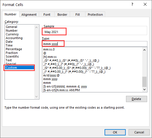
In this example, we’ve listed months in column E. These month values are actually dates formatted to omit the day, using custom number formatting.

The custom data format is “mmm yyyy” to show May 2021.

Sum by Month Over Multiple Years

The above example summed data with dates that fell within a specific month and year. Instead you can sum data with dates that fall within a month in any year using the SUMPRODUCT Function.

=SUMPRODUCT(C3:C8,--(MONTH(B3:B8)=MONTH(G3)))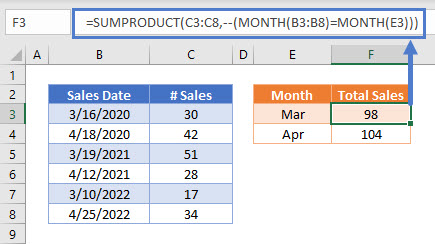

In this example, we use the SUMPRODUCT Function to perform complicated “sum if” calculations. Let’s walk through the formula.

This is our final formula:

=SUMPRODUCT(C3:C8,--(MONTH(B3:B8)=MONTH(G3)))

First, the SUMPRODUCT Function lists the Number of Sales for each Sales Date and then compares the month of each Sales Date against the specified Month, returning TRUE if the months match, or FALSE if they don’t:

=SUMPRODUCT({30;42;51;28;17;34},--({TRUE;FALSE;TRUE;FALSE;TRUE;FALSE}))

Next the double dashes (–) convert the TRUE and FALSE values into 1s and 0s:

=SUMPRODUCT({30;42;51;28;17;34},{1;0;1;0;1;0})

The SUMPRODUCT Function then multiplies each pair of entries in the arrays:

=SUMPRODUCT({30;0;51;0;17;0})

Finally, the numbers in the array are summed:

=98

More details about using Boolean statements and the “–” command in a SUMPRODUCT Function can be found here

Sum if by Month in Google Sheets

These formulas work exactly the same in Google Sheets as in Excel.