Sum If Date Range – Excel & Google Sheets

This tutorial will demonstrate how to use the SUMIFS Function to sum data falling within a specific date range in Excel and Google Sheets.

Sum Data by a Date Range

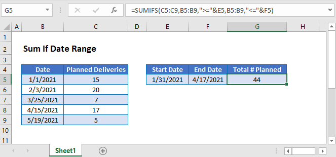
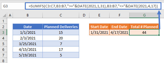
The SUMIFS Function sums data that meet certain criteria. In this example, we  sum Planned Deliveries if their Date is between 1/31/2021 and 4/17/2021, inclusive.

=SUMIFS(C3:C7,B3:B7,">="&DATE(2021,1,31),B3:B7,"<="&DATE(2021,4,17))

To start, we’ve hard-coded the dates directly into the SUMIFS Function using the DATE Function. When using this technique,

put operators within double quotes (e.g. “>=”). To join them with a function, use an ampersand (&). So, the criteria are:

• “>=”&DATE(2021,1,31) to set the start date and
• “<=”&DATE(2021,4,17) to set the end date.

Other Date Criteria

We can similarly use other logical operators to sum data. For example, if your dates are…

• equal to a certain date, use “=”&DATE(2021,4,15) OR DATE(2021,4,15).
• greater than a certain date, use “>”&DATE(2021,4,17).
• not equal to a certain date, use “<>”&DATE(2021,4,17).

Sum if Date Range – Cell References

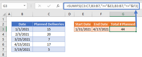
It’s not typically good practice to hard-code values into formulas. It’s more flexible to use separate cells to define the criteria instead. Below, we’ve entered the dates into separate cells and we join the cell references to the operators with &.

=SUMIFS(C3:C7,B3:B7,">="&E3,B3:B7,"<="&F3)

Locking Cell References

To make our formulas easier to read, we’ve shown the formulas without locked cell references:

=SUMIFS(C3:C7,B3:B7,">="&E3,B3:B7,"<="&F3)

But these formulas will not work properly when copy and pasted elsewhere with your Excel file. Instead, you should use locked cell references like this:

=SUMIFS($C$3:$C$7,$B$3:$B$7,">="&E3,$B$3:$B$7,"<="&F3)

Read our article on Locking Cell References to learn more.

Sum if Date Range in Google Sheets

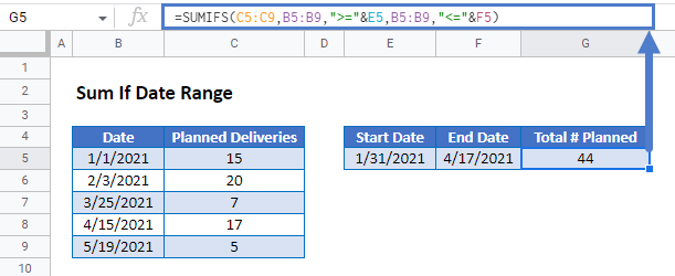
These formulas work exactly the same in Google Sheets as in Excel.