Sum If Between Two Values – Excel & Google Sheets

This tutorial will demonstrate how to use the SUMIFS Function to sum rows with data between two values in Excel and Google Sheets.

Sum if Between Numbers

The SUMIFS Function sums data rows that meet certain criteria. Its syntax is:

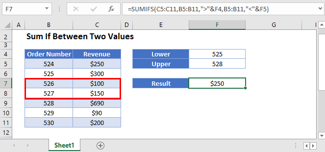
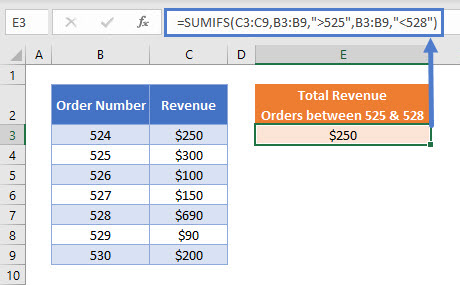
This example will sum the Revenue for all Order Numbers between (but not including) 525 and 528.

=SUMIFS(C3:C9,B3:B9,">525",B3:B9,"<528")

As you can see above, we use two logical tests as SUMIFS criteria:

• “>525” represents “greater than 525”
• “<528” represents “less than 528”

Note that when hard-coding criteria into the SUMIFS Function, the logical test must be within double quotes (“”).

If you wish to include the order numbers 525 and 528 in the formula, use the criteria:

">=525" and "<=528"

Sum If Between Numbers – Cell References

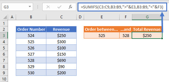
Usually, it is bad practice to hard-code values into formulas. Instead, it is more flexible to use separate cells to define the criteria.

=SUMIFS(C3:C9,B3:B9,">"&E3,B3:B9,"<"&F3)

Now we add the logical operators within double quotes (“”) and use the & symbol to join the operator with the value:

">"&E3 and "<"&F3

If you want to include the order numbers 525 and 528 in the formula, use the criteria:

">="&E3 and "<="&F3

Locking Cell References

To make our formulas easier to read, we’ve shown the formulas without locked cell references:

=SUMIFS(C3:C9,B3:B9,">"&E3,B3:B9,"<"&F3)

But these formulas will not work properly when copy and pasted elsewhere in your file. Instead, you should use locked cell references like this:

=SUMIFS($C$3:$C$9,$B$3:$B$9,">"&E3,$B$3:$B$9,"<"&F3)

Read our article on Locking Cell References to learn more.

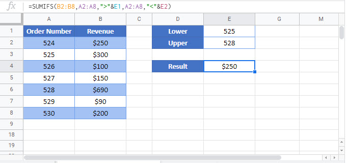
Sum If Between Values in Google Sheets

These formulas work exactly the same in Google Sheets as in Excel.