Reverse VLOOKUP – Right to Left – Excel & Google Sheets

This tutorial will demonstrate how to perform a “reverse VLOOKUP” in Excel and Google Sheets.

Reverse VLOOKUP – Right to Left

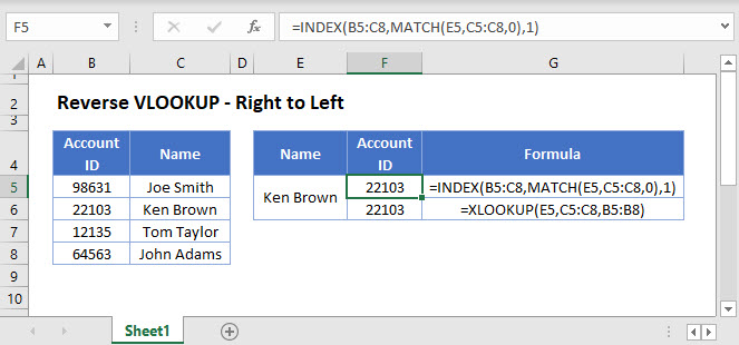
When you use the VLOOKUP function, the lookup column must be the left-most column in your data set. So you can only perform a lookup left to right.

However, you can work around this limitation by using the INDEX / MATCH combination (or the new XLOOKUP Function as you’ll see below).

=INDEX(B3:D6,MATCH(F3,C3:C6,0),1)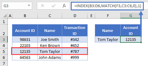

The formula works as follows:

MATCH Function

We use the MATCH function to return the relative position (i.e., the row number in the array) of the lookup item.

=MATCH(F3,C3:C6,0)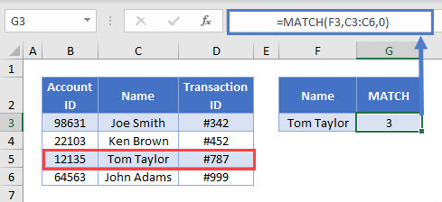

Think of the MATCH Function, as similar to a VLOOKUP performed on a single column, except instead of returning the value, the row number is returned instead.

INDEX Function

Once we have the row number, we use the INDEX Function to return the value from that row number.

=INDEX(array, row_num,[column_num])

=INDEX(B3:D6,G3,1)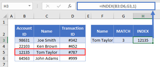

The INDEX Function returns the cell value of a certain row and column in your range. The MATCH Function supplies the row number. We set the column number to be 1 because we want the first column of data.

Combining the functions, gives us our original formula:

=INDEX(B3:D6,MATCH(F3,C3:C6,0),1)

XLOOKUP Function

The XLOOKUP Function was introduced after Excel 2019 to Office 365 users. The XLOOKUP Function also allows you to perform a reverse lookup:

=XLOOKUP(F3,C3:C6,B3:B6)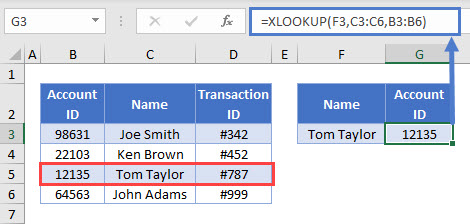

Reverse VLOOKUP Right To Left in Google Sheets

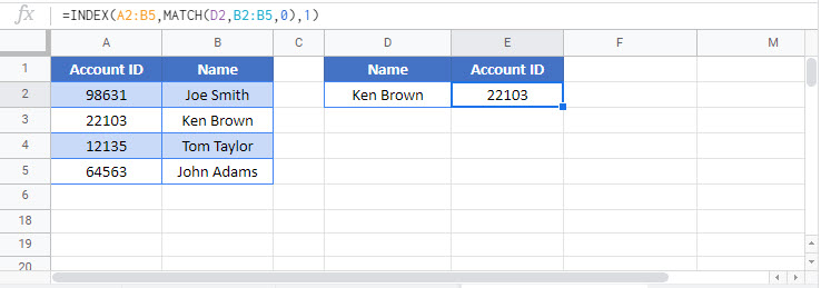
These formulas work exactly the same in Google Sheets as in Excel.