How to Remove Non-Numeric Characters – Excel & Google Sheets

This tutorial will demonstrate you how to remove non-numeric characters from cells in Excel and Google Sheet.

Remove Non-Numeric Characters

Note: The functions mentioned in this article were introduced in Excel 2016. If you have an older version of Excel, please see this article: Find & Extract Number from String.

With the TEXTJOIN, SEQUENCE, MID, and IFERROR Functions you can remove all non-numeric characters:

=TEXTJOIN("",TRUE,IFERROR(MID(B3,SEQUENCE(LEN(B3)),1)+0,""))

Let’s see how this formula works.

The SEQUENCE and LEN Functions return an array of numbers starting from 1 to the length of our alphanumerical string. In our case it will be {1,2,3,4,5,6,7,8,9,10,11,12,13}.

=TEXTJOIN("",TRUE,IFERROR(MID(B3,{1;2;3;4;5;6;7;8;9;10;11;12;13},1)+0,""))

The MID Function returns the characters corresponding to the positions from our numerical array above:

=TEXTJOIN("",TRUE,IFERROR({"1";"3";"M";"o";"n";"d";"a";"y";"0";"1";"D";"a";"y"}+0,""))

Adding 0 to each item in the array will cause an error if the value is text. Then the IFERROR Function will replace the error with a blank string, leaving only the numerical values:

=TEXTJOIN("",TRUE,{1;3;"";"";"";"";"";"";0;1;"";"";""})

Last, the TEXTJOIN Function returns only the numerical characters.

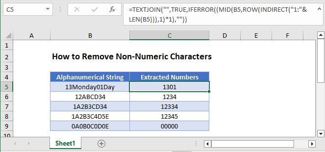
Instead of using the SEQUENCE function, you can achieve the same goal by combining the TEXTJOIN function with the LEN, INDIRECT, ROW, MID and IFERROR functions.

=TEXTJOIN("",TRUE,IFERROR((MID(B3,ROW(INDIRECT("1:"&LEN(B3))),1)*1),""))

How to Remove Non-Numeric Characters in Google Sheets

All the examples explained above work the same in Google sheets as they do in Excel.