Rank If in Excel & Google Sheets

This tutorial will demonstrate how to calculate “rank if”, ranking items in a list based­­ on criteria.

RANK IF Formula

Excel does not provide a “RANKIF” Function. Instead, you can use the COUNTIFS Function to “rank if”.

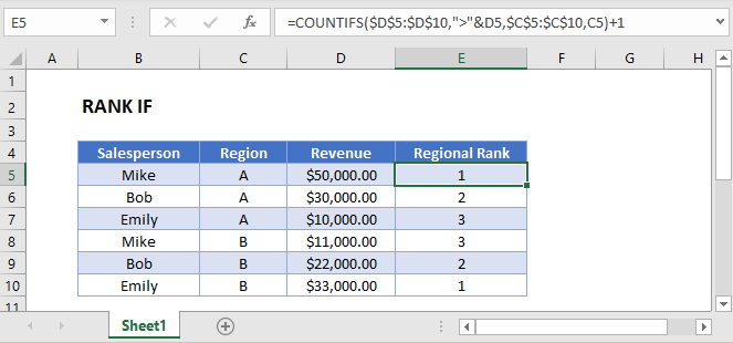
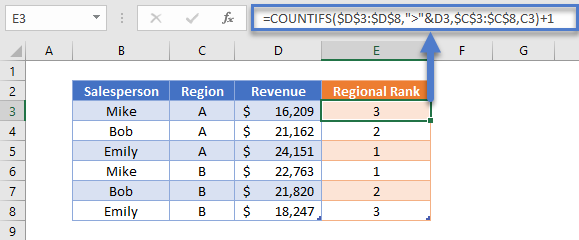
This example will rank the salespersons by revenue for each region separately:

=COUNTIFS(D3:D8,">"&D3,C3:C8,C3)+1

How Does the Formula Work?

The COUNTIFS Function counts cells with values that meet specific criteria. To calculate “rank if”, we will use two criteria:

1. Count only the values that are greater than the current row’s value. (This is where the “ranking” occurs).
2. The condition (or conditions) that you want to apply.

Note: the “+1” at the end of the formula is required to start the ranking at 1 instead of 0.

Reverse RANK IF Formula

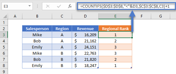
In the previous examples, we ranked Salespersons by revenue from largest to smallest.

To rank the salespersons by revenue in reverse order, simply switch the sign in the first criteria to be less than “<” instead.

=COUNTIFS(D3:D8,"<"&D3,C3:C8,C3)+1

Locking Cell References

To make our formulas easier to read, we’ve shown the formulas without locked cell references:

=COUNTIFS(D3:D8,">"&D3,C3:C8,C3)+1

But these formulas will not work properly when copy and pasted elsewhere with your Excel file.

=COUNTIFS($D$3:D8,">"&$D$3,$C$3:$C$8,C3)+1

Read our article on Locking Cell References to learn more.

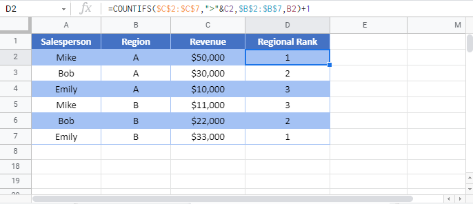
Rank If in Google Sheets

All the examples explained above work the same in Google sheets as they do in Excel.