Max If (Max Value with Condition) – Excel & Google Sheets

This tutorial will demonstrate how to find the largest value which meets specific conditions in Excel and Google Sheets.

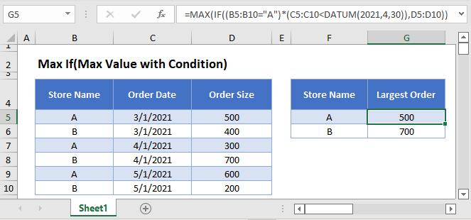
MAXIFS Function

Users of Google Sheets and Excel 2019 or later can use the single MAXIFS Function .

This example uses the MAXIFS and DATE Functions to show the largest Order Size for each Store Name for Order Dates before 4/30/2021:

=MAXIFS(D3:D8,B3:B8,"A",C3:C8,"<"&DATE(2021,4,30))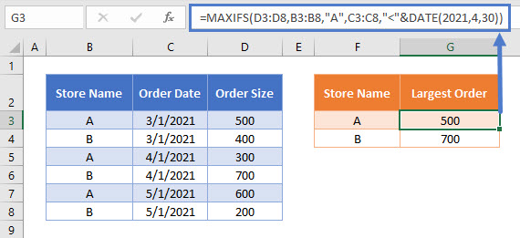

The MAXIFS Function does not require the user to press CTRL + SHIFT + ENTER when entering the formula.

Max If Array Function

If you don’t have access to the MAXIFS Function, you can create an Array Formula to simulate the MAXIFS Function. We will walk through this below.

The MAX Function identifies the largest value in a series of numbers.

=MAX(B2:B11)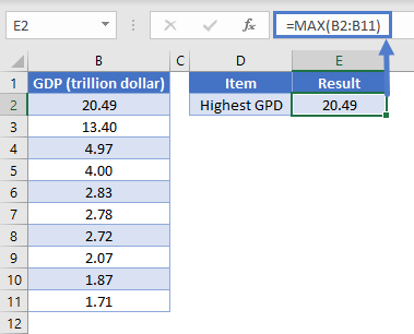

We can use the MAX Function combined with an IF Function to identify the largest value that meets a specified condition.

This example will use the MAX and IF Functions in an array formula to identify the largest Order Size for each Store Name

{=MAX(IF(B3:B8="A",D3:D8))}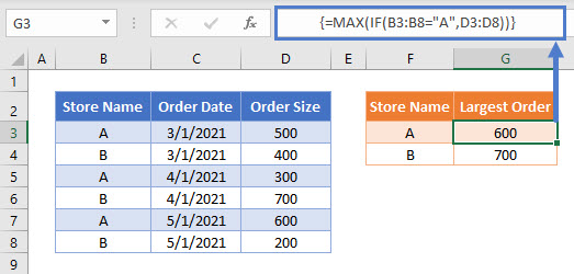

In Office 365 and versions of Excel after 2019, you can simply enter the above formula like you normally would (by pressing ENTER).

However, for Excel 2019 and earlier you must enter the formula by pressing CTRL + SHIFT + ENTER. After doing so, you’ll notice curly array brackets appear around the formula.

To show how this formula works, let’s break it down into steps.

This is our final formula (shown without the automatically added array formula brackets):

=MAX(IF(B3:B8="A",D3:D8))

First, the cell range values are added to the formula as arrays:

=MAX(IF({"A"; "B"; "A"; "B"; "A"; "B"}="A",{500; 400; 300; 700; 600; 200}))

Next the Store Name =”A” condition produces an array of TRUE/FALSE values:

=MAX(IF({TRUE; FALSE; TRUE; FALSE; TRUE; FALSE},{500; 400; 300; 700; 600; 200}))

Then the IF Function changes all TRUE values into the relevant Order Size:

=MAX({500; FALSE; 300; FALSE; 600; FALSE})

The MAX Function identifies the largest number in the array, whilst ignoring any FALSE values, to show the largest Order Size for the Store Name = “A”:

=600

Max If – Multiple Criteria

We can also identify the largest value based on multiple criteria by using Boolean logic.

This example will show the largest Order Size for each Store Name, but for Order Dates before 4/30/2021 by using the MAX, IF and DATE Functions:

{=MAX(IF((B3:B8="A")*(C3:C8<DATE(2021,4,30)),D3:D8))}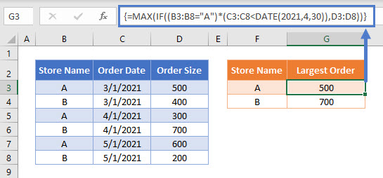

Notice here we multiply two sets of TRUE/FALSE criteria together:

(B3:B8="A") * (C3:C8<DATE(2021,4,30))

If both criteria are TRUE then the total condition will calculate as TRUE, but if one (or more) criteria is FALSE it will calculate as FALSE.

Using this methodology, it is possible to add many different criteria to this formula.

Max If – Multiple Criteria with Cell References

Usually, it is not good practice to hard-code values into formulas. Instead, it’s more flexible to use separate cells to define the criteria.

To match the Store Name to the value shown in column F, we can update the formula to be:

{=MAX(IF((B3:B8=F3)*(C3:C8<DATE(2021,4,30)),D3:D8))}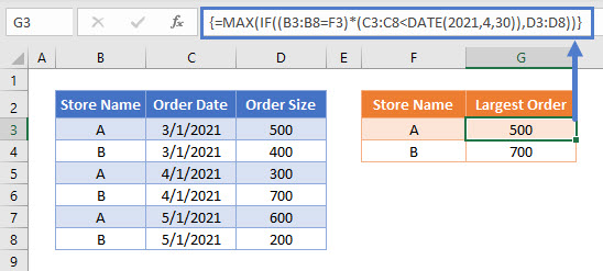

Locking Cell References

To make our formulas easier to read, we’ve shown the formulas without locked cell references:

{=MAX(IF((B3:B8=F3)*(C3:C8<DATE(2021,4,30)),D3:D8))}

But these formulas will not work properly when copy and pasted elsewhere in your file. Instead, you should use locked cell references like this:

{=MAX(IF(($B$3:$B$8=F3)*($C$3:$C$8<DATE(2021,4,30)),$D$3:$D$8))}

Read our article on Locking Cell References to learn more.

 

Max If (Max Value with Condition) in Google Sheets

The examples shown above work exactly the same in Google Sheets as in Excel, but as the MAXIFS Function is available, it is recommended to use this single function instead of combining the MAX and IF Functions.

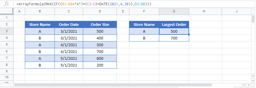
If you do want to use the MAX / IF Array Formula, then enter the formula within the ARRAYFORMULA Function (Or simply use CTRL + SHIFT + ENTER and Google Sheets will add this function for you).

=ARRAYFORMULA(MAX(IF((B3:B8="A")*(C3:C8<DATE(2021,4,30)),D3:D8)))